
The role of radio frequency identification (RFID) technologies in improving garment assembly line operations
Z.X. Guo, Sichuan University, China
W.K. Wong, S.Y.S. Leung, J.T. Fan and S.F. Chan, The Hong Kong Polytechnic University, Hong Kong
Abstract:
In this chapter, a production control problem on a flexible assembly line (FAL) with flexible operation assignment and variable operative efficiencies is described. A mathematical model of the production control problem is formulated by considering the time-constant learning curve to deal with the change of operative efficiency in real-life production. An intelligent production control decision support (PCDS) system is developed, composed of a radio frequency identification (RFID) technology-based data capture system and a PCDS model comprising a bi-level genetic optimization process, and a heuristic operation routing rule is developed. Experimental results demonstrated that the proposed PCDS system could implement effective production control decision-making.
Key words
production control; decision support system; flexible assembly lines (FALs); genetic algorithms (GAs); learning curves
5.1 Introduction
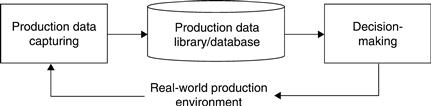
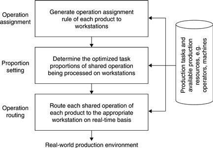
Effective production control is useful and necessary to improve production and management performances and reduce the running costs of factories. A generic architecture for production control decision-making is shown in Fig. 5.1. In a real-life production environment, production data on production orders, production quantities of each workstation and the whole production line, operative efficiency, etc., are collected from shop floors or assembly lines by using various types of data capture methods, including the manual recording method, barcode scanning, and the most updated radio frequency identification (RFID) technology. Based on the collected production data, the production manager makes decisions to achieve various production objectives.
On shop floors or assembly lines with a low level of automation, it is impossible to obtain real-time production data owing to the absence of an effective data capture system. Thus, it is also impossible to make accurate and real-time decisions for production control. This chapter presents an intelligent production control decision support (PCDS) system, which is integrated with an RFID-based real-time data capture system, to assist in the production control decisions on a flexible assembly line (FAL).
5.2 Key issues in developing flexible assembly lines (FALs)
To meet increasingly fierce market competition, more manufacturing enterprises seek benefits from manufacturing flexibility and effective production control. Beach et al. (2000) provide a comprehensive review of manufacturing flexibility. There are various types of manufacturing flexibility, such as machine flexibility and routing flexibility. Machine flexibility is measured by the number of operations that a workstation processes and the time needed to switch from one operation to another. The more operations a workstation processes, the less time switching takes and the higher the machine flexibility becomes. Routing flexibility is the ability of a production system to manufacture a product using several alternative routes in the system and is usually determined by the number of such potential routes.
The FAL is an increasingly attractive assembly form for small- or mid-scale production in many industries. Unlike the traditional assembly line, some FALs allow flexible operation assignment, where one operation can be assigned to multiple workstations for processing, and multiple operations can be assigned to the same workstation. When one operation is assigned to multiple workstations, the processing of this operation is shared by the assigned workstations and is taken as a shared operation. Each shared operation of a product should be routed to an appropriate workstation on a real-time basis. Obviously, the FAL with flexible operation assignment involves machine flexibility and routing flexibility. In practice, this type of FAL is normally used in apparel manufacturing.
5.2.1 Variability of operative efficiency
On a highly automated assembly line, the efficiency to process a certain task is deterministic. Yet for FALs with a low level of automation, for example, FALs highly relying on manual effort, the operative efficiency of each task is seldom constant. The variable operative efficiency leads to fluctuation of the cycle time and increases the complexity of production control. In the field of production control, some researchers assume that the task time is an independent normal variable (Gamberini et al., 2006; Moodie and Young, 1965; Suresh and Sahu, 1994). Some other researchers also assume task times with different probability distributions (Arcus, 1966; Nkasu and Leung, 1995). However, the stochastic change of the task time cannot reflect the increasing efficiency of the operator caused by repetitive and cumulative operations, and the random probability distribution cannot reflect the increasing trend of operative efficiency owing to learning effects.
Thorndike (1898) and Thurstone (1919) scientifically analyzed the learning phenomenon by focusing on the human subject’s behavior and concluded that the time required for executing a specific task decreased with the cumulative experience. Some years later, learning curves were presented and widely used to describe the relationship between the operative efficiency and the accumulated operating time.
Wright (1936) established the first and most common learning curve model in 1936, which indicates that a given operation is subject to a 20% productivity improvement each time the production quantity doubles, but this curve has a significant deficiency because its asymptote is zero. After Wright’s curve, various learning curve models have since been developed (Badiru, 1992), such as de Jong’s equation, Wiltshire’s equation and the time-constant model. On the basis of an in-depth comparison of a number of models, Hackett (1983) concluded that the time constant model (Bevis, 2004; Hitchings, 1972) is the most practical model for general use, because it can fill a wide range of observed data.
However, limited work has been done to investigate the production control problem with learning effects (Mosheiov and Sidney, 2003; Wang and Xia, 2005). The learning effect on production control decision-making for FALs has not yet been considered. For FALs that are highly reliant on manual effort, it is not unusual for many newly trained operators to be assigned to run complicated operations owing to labor shortage. Thus, it is necessary and important to consider these learning effects.
5.2.2 Production control decision-making
Research on the PCDS system has received little attention, although various decision support systems have been developed for a wide range of applications (Anon, 2007; Epic Data Inc., 2007; MSC Limited, 2007). Traditionally, the decision-making for production control relies on the experience and simple interpretation of production managers and supervisors. However, human decisions tend to be subjective, late, inconsistent and even inaccurate owing to the complexity of production decision-making problems. A large number of studies have investigated production control of the basis of two types of problems: production scheduling and assembly line balancing. Production scheduling involves mainly shop scheduling problems (Cheng et al., 1999; Framinan et al., 2004; Shakhlevich et al., 2000) and flexible manufacturing system scheduling (Chan and Chan, 2004; Sawik, 2002). Assembly line balancing involves mainly simple (Baybars, 1986; Scholl and Becker, 2006) and generalized assembly line balancing problems (Becker and Scholl, 2006). However, no existing literature is available on the production control and decision support system for the FAL in terms of flexible operation assignment and variable operative efficiencies.
The developed methodologies for decision support of production control involve a wide range of optimization techniques such as:
• simulation-based techniques (Chan and Chan, 2004; Chong et al., 2003);
• classical optimization techniques (Crauwels et al., 2005; Ibraki and Nakamura, 1994); and
• intelligent optimization algorithms (Cheng et al., 1999; Guo et al., 2008).
Due to the NP-hard nature of most production control problems (Gutjahr and Nemhauser, 1964), intelligent algorithms with heuristic optimization capacity are widely adopted (Charalambous and Hindi, 1991; Guo et al., 2008; Scholl and Becker, 2006), while the genetic algorithm (GA) is a typical representative due to its capability of global optimization. However, none of the algorithms are applicable to any other production control problems without adjustment or modification. Moreover, due to the absence of real-time and accurate production data, most of the developed methodologies cannot be used in real-life production control.
In recent years, as the application of the RFID technology has become economically feasible, some RFID-based data capture systems have been developed to obtain real-time and accurate production data and their effectiveness has also been proved by various industrial applications and practices. With the support of effective data capture technology, it is feasible, in theory and also in practice, to develop an effective PCDS system to assist in production management for the decision-making process of production control.
In this study, the production control problem on an FAL with flexible operation assignment and variable operative efficiencies is investigated. The learning curve theory is used in this system to represent the change of operative efficiency with accumulated operating time. A GA-based intelligent PCDS system integrating with an RFID-based real-time data capture system was proposed to provide effective production decisions, which could meet the desired cycle time of each production order and minimize the total idle time on the FAL.
Section 5.2 of this chapter formulates the production control problem on an FAL and describes the variable operative efficiency based on the learning curve theory. Section 5.3 describes the GA-based intelligent PCDS system to solve the addressed problem in detail. Experiments and discussions are presented to validate the effectiveness of the proposed system in Section 5.4. Finally, the study is summarized and further research is suggested in Section 5.5.
5.3 Modelling flexible assembly lines (FALs)
In this study, the FAL is composed of a number of workstations including different types of machines. Each workstation is a physical location that accommodates an operator, a machine and a buffer. Several production orders with given quantities representing different product types are executed on the FAL. Each order comprises a series of manual operations. According to the pre-determined processing sequence, operations involved in each order must be processed in their corresponding workstations. On the FAL, one operation can be assigned to multiple workstations, while one workstation can also perform multiple operations simultaneously. The objective of production control is to meet the desired time cycle of each order and minimize the total idle time of all workstations on the FAL, by assigning and routing each operation to the most appropriate workstation or operator. In this study, it is assumed that the operation of a product cannot be interrupted once it starts. The efficiency of each operator between different operations is independent.
5.3.1 Notations
The following notation is utilized in developing the mathematical model of the production control problem addressed in this research:
1. Parameters:
Pi, ith production order, 1 ≤ i ≤ p
Oij, jth operation of order Pi
Mkl, lth machine (workstation) of the kth machine type
STij, standard time of operation Oij, the time to complete operation Oij of one product with 100% operative efficiency
ηijkl, task proportion (weight) of operation Oij being performed on machine Mkl, 0 ≤ ηijkl ≤ 1
SOkl, a set of operations, which can be processed on machine Mkl
EMijkl, operative efficiency of operation Oij on machine Mkl, which is a variable in the real-life production process
DCTi, desired cycle time of order Pi, the desired time interval of consecutive products entering the assembly line
ACTi, actual cycle time of order Pi, the actual time interval of consecutive products entering the assembly line
αi, penalty weight for order Pi when its actual cycle time is less than its desired cycle time
βi, penalty weight for order Pi when its actual cycle time is greater than its desired cycle time
AMi, a set of workstations processing order Pi
Ni, the number of workstations processing order Pi
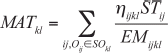
MATkl, average assembly time of each product on machine Mkl
SMij, a set of machines which can handle operation Oij
Cij, completion time of operation Oij
ETij, elapsed time between operation Oij and its latter operation including the transportation time and the set-up time
Si′j′, starting time of operation Oi′j′
PR(Oi′j′, a set of the preceding operations of operation Oi′j′
Tij, time for processing operation Oij.
2. Variables:
Xijkl, binary variable, Xijkl is equal to 1 if operation Oij is assigned to machine Mkl, otherwise it is equal to 0.
λi,. binary variable, λi is equal to 1 if actual cycle time ACTi is less than the desired cycle time DCTi, otherwise it is equal to 0.
5.3.2 Mathematical model
The addressed problem minimizes two objectives and its mathematical model is described as follows:
Minimize:
![]() [5.1]
[5.1]
and
![]() [5.2]
[5.2]
where
 [5.3]
[5.3]
subject to
![]() [5.4]
[5.4]
![]() [5.5]
[5.5]
![]() [5.6]
[5.6]
![]() [5.7]
[5.7]
![]() [5.8]
[5.8]
Objective function (1) is to satisfy the desired cycle time of each order, and objective function (2) is to minimize the total idle time of all workstations on the FAL. Constraint (3) indicates that operation Oij can only be operated by workstations which can handle it. Constraint (4) indicates that each workstation must process at least one operation. Constraint (5) denotes that each operation of one product must be processed. Constraint (6) indicates that each operation of one product cannot be started before its preceding operation is completed and the time-out between the two operations elapses. Constraint (7) indicates that operation Oij must be assigned with the processing time.
5.3.3 Learning-curve-based operative efficiency
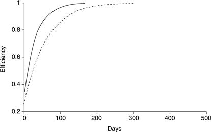
The operating time of operation Oij in workstation Mkl is equal to its standard time STij divided by the current efficiency EMijkl of the operator in workstation Mkl. The operative efficiency EMijkl differs between different products, owing to the increase in the accumulated operating time. In this study, the operative efficiency is represented by the time-constant learning curve model (Bevis, 2004; Hitchins, 1972), which is defined by
![]() [5.9]
[5.9]
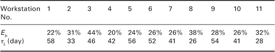
where EL(tL) is the predicted operative efficiency at time tL, Eb is the initial efficiency of the operator, EΔ is the maximal improvement in performance due to learning, and τL is the model time constant, which is a measure of how quickly the performance improvement is achieved. The ultimate efficiency of each operator is assumed to be 100% (i.e. = 1 at tL → ∞. EΔ = 1 – Eb), and each day has 8 working hours. Figure 5.2 shows the changing trends of two learning curves with different Eb and τL
5.4 Intelligent decision support system for production control on flexible assembly lines (FALs)
An intelligent PCDS system, which can help achieve effective and real-time production control decision-making on the FAL under investigation, is introduced in this section (Fig. 5.3).
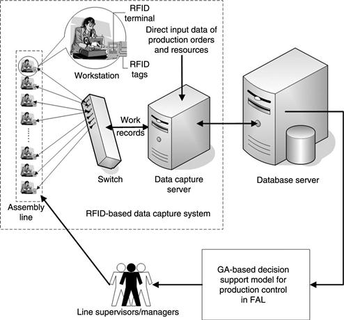
5.4.1 System architecture
As shown in Fig. 5.3, the system is composed of an RFID-based data capture system, a database server and a GA-based decision support model. The RFID-based data capture system collects all real-time job processing records and production data from the FAL. It is composed of RFID tags, RFID terminals, switches and data capture servers. In each workstation, an RFID terminal is installed, which can collect the job processing records by reading RFID tags attached to each batch of work-in-progress. The terminal can also display the historical job records to the operator. The terminals of each assembly line are connected to form a network by the switch. The switch is a device that channels incoming data from any of the multiple input ports to a specified output port that takes the data toward its intended destination, which is connected with a data capture server. The data communication uses the TCP/IP protocol. The data capture server collects production data based in two ways and saves them into the database.
First, the given data on production orders, workstations and assembly operators are input directly by the computer operator. Second, during the production process, each operator reads the RFID tag being attached to each batch of work-in-progress using the RFID terminal after finishing an operation. The job records from the RFID terminals are input by Ethernet. However, the data capture server also reads production information from the database and displays it on the RFID terminals. On the basis of the real-time production data stored in a database server using MySQL, Ms SQL Server or Oracle according to different requirements for data processing, the decision support model generates effective solutions to production control of the FAL. The recommended solutions are implemented by the assembly line supervisors or managers through assigning and routing operations of each product to the determined workstation on a real-time basis.
The GA-based decision support model is the kernel of the system (Fig. 5.4). As shown in the decision support model of the figure, the decision support for production control of the FAL is implemented according to the following procedures:
• Procedure 1: Assign flexibly operations of each type of product to different operations. One operation can be assigned to multiple workstations and multiple operations can be assigned to the same workstation. This optimized operation assignment can be implemented by a genetic optimization process with an operation-based representation.
• Procedure 2: Determine the optimal task proportions of each shared operation being processed in different workstations, which can be implemented by using a real-coded GA.
• Procedure 3: According to the optimized operation assignment results and task proportions of each shared operation, route operations of each product to the appropriate workstation on a real-time basis, which can be implemented by using a heuristic routing rule.
For each operation assignment solution in the first procedure, the second procedure seeks the optimal task proportions of each shared operation. In other words, the solution to the second procedure relies on the solution to the first procedure. It is a typical bi-level optimization problem. In this study, the bi-level GA (BiGA) presented by Guo et al. (2008) is modified to implement the two procedures. In the BiGA, a novel representation and modified genetic operators are presented to deal with the flexible operation assignment.
5.4.2 Modified bi-level genetic algorithm
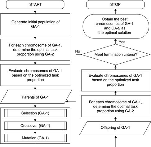
The modified BiGA (mBiGA) is also composed of two genetic optimization processes (GA-1 and GA-2) (Fig. 5.5). In the mBiGA, GA-1 generates the optimal operation assignment to workstations, in which the representation and genetic operators are the same as those in GA-1 of the BiGA (Guo et al., 2008). Based on each chromosome of GA-1, GA-2 determines the task proportions (weights) of the shared operation being processed in different workstations. Seeking the optimal task proportions (weights) is a first-order multivariate function optimization problem, which can be optimized by a GA with real-coded representation. The following processes of the BiGA are different from those of the mBiGA:
1. Representation in GA-2: each gene represents the task proportion of an operation assigned to the corresponding workstation. By considering the assignment of n operations, nmij denotes the number of machines allocated to process operation Oij and PSij denotes the summation of nmij-1 weights of Oij The number of genes in each chromosome of GA-2 is the summation of nmij minus n, since the nmthij weight is equal to 1-PSij.
2. Initialization in GA-2: the initial population is generated by initializing each task proportion (weight) randomly in the chromosome between 0 and 1, based on the premise of PSij ≤ 1.
3. Fitness function: the fitness function of GA-1 is the same as that of GA-2.
The objective of addressing the production control problem is to satisfy the desired cycle time of each order and minimize the total idle time of all workstations, which can be defined by
![]() [5.10]
[5.10]
where wz and wIT are the relative weights placed upon the objectives Z(Xijkl) and IT(Xijkl), respectively. The less the weighted summation of the two objectives, the greater the fitness becomes. The fitness function ft can be defined as:
![]() [5.11]
[5.11]
Based on the chromosomes in GA-1 and GA-2, the fitness should be calculated in each generation. In this study, the operative efficiency of the operator is variable and affected by the learning phenomenon. Therefore, the operative efficiency of one operator processing the same operation differs between different production cycles. It is assumed that the order size (product quantity) of order Pi is OSi and the number of assembly operation is Ui. The chromosomes in GA-1 and GA-2 are given. On the basis of chromosomes of GA-1 and GA-2, the procedure to calculate fitness is described in detail as follows:
1. Parameter initialization: order index i = 1;
2. Parameter initialization: for order Pi, initialize product index u = 1, operation index v = 1, production days iDays = 0;
3. For operation v of the uth product, select an operator (operator w) to process it according to the corresponding assignment rule and the operator’s task proportion assigned;
4. For operator w, calculate his/her operating time for processing the operation v of the current product:
i. Calculate his/her accumulated operating time AccT1 for processing operation v;
ii. Calculate his/her accumulated operating time AccT2 on the current day;
5. If AccT2> 8*3600 (working time in second unit per day), then iDays = iDays + 1, AccT2 = 0;
6. v = v + 1. If v > Ui, then go to (7), otherwise go to (3);
7. u = u + 1. If u > OSi, then go to (8), otherwise set v = 1 and go to (2);
8. On the basis of the accumulated operating time AccT1 of each operation, calculate the actual cycle time of order Pi and the idle time of workstations processing order Pi;
9. i = i + 1. If i is greater than the number of orders, i.e. i > p, then go to (10), otherwise go to (1);
10. On the basis of the actual cycle time of all orders and the total idle time of all workstations, calculate the fitness.
5.4.3 Operation routing rule
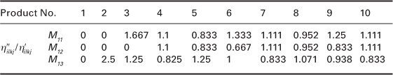
After the preceding operations of the shared operation of a product are completed, the next step is to route the shared operation to an appropriate workstation based on the optimized operation assignment and task proportions of the shared operation being processed in different workstations. Assuming that operation Oij is assigned to m machines (Mk1, Mk2, … Mkm) according to the optimized operation assignment, η′ijkl denotes the optimized task proportion that operation Oij should be processed on machine Mkl(η′ijkl > 0), η″ijkl denotes the task proportion that operation Oij has been processed on machine Mkl and Qijkl denotes the number of operation Oij, which has been assigned to machine Mkl. For shared operation Oij. of a product, the heuristic operation routing rule is described in the following procedure:
1. Calculate ![]() for machine Mkl (for the first product, set η″ijkl = 0).
for machine Mkl (for the first product, set η″ijkl = 0).
2. Calculate η″ijkl/η′ijkl for each machine Mkl.
3. Assign operation Oij of the current product to the machine Mkl with the minimum η″ijkl/η′ijkl. If multiple machines have the same minimum value, one of the machines will be chosen randomly.
Table 5.1 shows an example of the operation routing to process operation O11 of 10 units of the same product. Operation O11 is assigned to machines M11, M12 and M13. The task proportions of operation O11 to be processed on these three machines are 0.3, 0.3 and 0.4 respectively, generated by the proposed mBiGA. The rows of η″ijkl/η′ijkl describe the current value η″ijkl/η′ijkl of operation O11 of each product in the relevant machine, and the shaded grid represents that the corresponding machine is selected to process the operation of the corresponding product. According to the results of operation routing (Table 5.1), operation O11 of the first unit of the product is assigned to M11, that of the second unit of the product is assigned to M13, etc. After the 10 units of the product are completed, the actual task proportion processed on each machine is equal to the optimized task proportion.
5.5 Testing the effectiveness of the intelligent production control decision support (PCDS) system
To validate the effectiveness of the proposed intelligent PCDS system for production control of the addressed FAL, a series of experiments were conducted. This section presents the details of these experiments and examines the effect of the learning phenomenon on production control decision-making. In these experiments, assume there is no shortage of materials, workstation breakdown or operator absenteeism on the FAL. The FAL discussed is empty initially. In other words, there is no work-in-process in each workstation.
5.5.1 Experiments
Under normal conditions, the operative efficiency of each operator increases with the increase in the accumulated operating time on the FAL due to the accumulated learning effect. To investigate the influence of efficiency increase on production decisions, two orders of different product quantities based on two different cases were executed in each experiment. In Case 1, 1000 products were made, while 5000 products were made in Case 2. In each experiment, the two orders were scheduled for production and the basic data for the orders are listed as follows:
1. Experiment 1: the desired cycle time of both orders 1 and 2 was 400 s. The product’s assembly process of Order 1 was from operations 1 to 7, and Order 2 was from operations 8 to 12.
2. Experiment 2: the desired cycle time of Orders 1 and 2 was 55 and 130 s, respectively. The product’s assembly process of Order 1 was from Operations 1 to 6, and Order 2 was from Operations 7 to 11.
3. Experiment 3: the desired cycle time of both orders was 50 s. The assembly operations of the two orders were the same as those in Experiment 2.
4. Experiment 4: the desired cycle time of Orders 1 and 2 was 70 and 225 s, respectively. The product’s assembly process of Order 1 was from Operations 1 to 5, and Order 2 was from Operations 6 to 10.
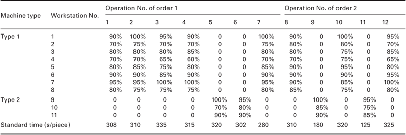
The experiments were conducted on an FAL with 11 workstations, Workstations 1 to 8 used machines of type 1 and workstations 9 to 11 used machines of type 2. The operative efficiency of each workstation depended on the type of machine, the skill level and the recent performance of the operator. The operative efficiencies in the four experiments are shown in Tables 5.2 to 5.5. The efficiency is set at 0 if the operator cannot process the corresponding operation. The standard time of each operation in the experiments is shown in the last rows of Tables 5.2 to 5.5. The processing time of operation Oij in workstation Mkl is equal to the standard time of this operation divided by its operative efficiency in workstation Mkl.
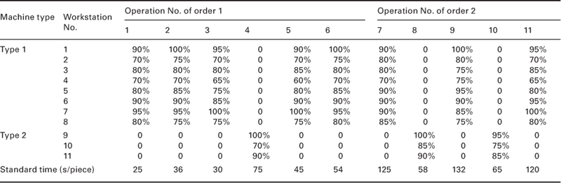
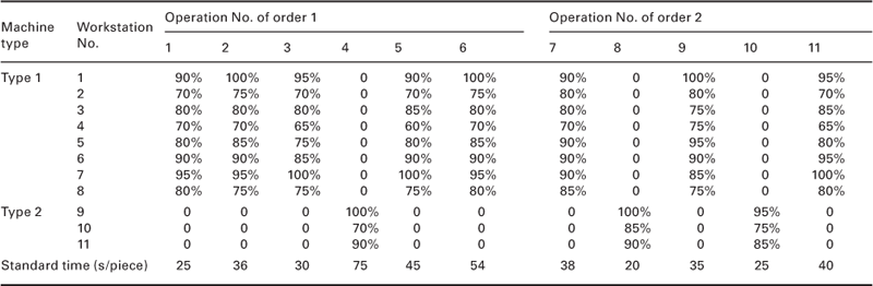
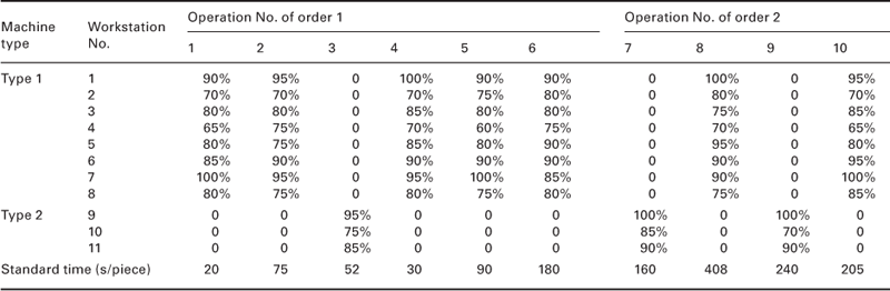
In this study, the learning curves of different operators were probably different and each operator had only one learning curve for different operations. That is, whichever operation was processed, the learning curve of the operator was the same. The parameters of the learning curves of each operator are shown in Table 5.6.
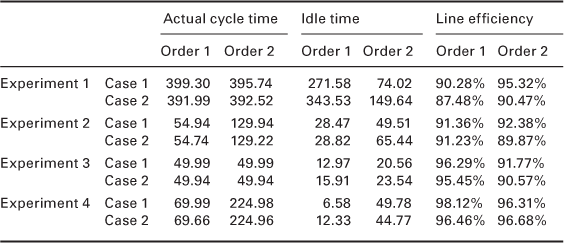
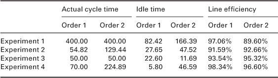
The production control solutions to the four experiments generated by the proposed PCDS system are shown in Tables 5.7 and 5.8. In Table 5.7, the first row represents the machine type, the second shows the workstation number, and other rows show the optimized operation assignment and task proportions of different experiments to the workstation. The first value of each cell represents the operation number and the value in the bracket represents the task proportion ηijkl of the operation being processed in the corresponding workstation. For example, the value 10(1) in the row of ‘Case 1 of Experiment 1’ shows that workstation 2 processes the whole (100%) of Operation 10, and the value (5(0.13),6(1)) shows that workstation 9 processes 13% of Operation 5 and 100% of Operation 6. In Table 5.8, the columns of ‘Actual cycle time’ show the optimized actual cycle time (seconds) of Orders 1 and 2 in four experiments, whereas the columns of ‘Idle time’ and ‘Line efficiency’ show the optimized average idle time (seconds) in each cycle and the optimized line efficiencies of Orders 1 and 2 in the four experiments. In this study, the line efficiency of order Pi is defined as the average processing time of workstations processing this order in each cycle divided by the actual cycle time of this order.
Table 5.7
Optimized operation assignment and task proportions of four experiments (with learning effects)
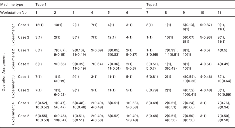
As shown in Table 5.7, the proposed mBiGA can implement flexible operation assignments, including assigning one operation to different workstations and multiple operations to the same workstation. For instance, in Case 1 of Experiment 2, Operation 7 is assigned to workstations 2 and 8, while Operations 7 and 9 are assigned to workstation 2. At the same time, the different task proportions of the shared operation are also optimized. For instance, in Case 1 of Experiment 2, the processing of Operation 7 is shared in workstations 2 and 8 and the task proportions are 0.67 and 0.33, respectively. In different cases of each experiment, the operation assignments are different because the quantities of the processed products are different.
Table 5.7 indicates that the actual cycle time of two orders are close to the desired cycle time in each case and the assembly line efficiency is also very good, which is between 87.48 and 98.12%. For instance, for Case 1 of Experiment 4, the actual cycles of Orders 1 and 2 are 69.99 and 224.98, respectively, that is their percentage errors are only 0.014 and 0.009%, respectively. For Order 1, the total idle time of all workstations in each cycle is only 6.58, which is less than 9.4% of its cycle time. The production flow of this order is thus very smooth. These results demonstrate that the proposed decision support system can solve the addressed production control problem effectively.
Table 5.8 shows that the actual cycle time of each order in Case 2 is less than that in Case 1. The operative efficiency of operators increases with the increase in the accumulated operating time. Therefore, in Case 2, more operating time is accumulated, leading to higher operative efficiency and lower cycle time.
5.5.2 Influence of different initial operative efficiencies
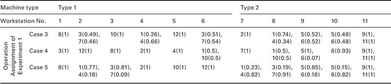
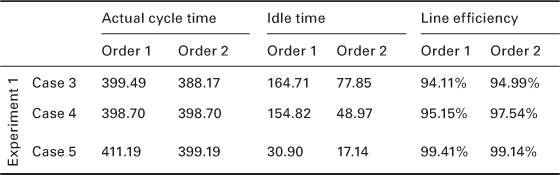
In this section, experimental Cases 3 to 5 are presented for the investigation of different initial operative efficiencies. The data of the three cases are the same as those of Case 2 of Experiment 1, except for the operative efficiencies of each operator. In Cases 3 to 5, the initial operative efficiencies of each operator are equal to his/her operative efficiencies (Table 5.2) multiplied by 90, 80 and 70%, respectively. For instance, the efficiencies of the operator of workstation 1 processing Operations 1 to 3 should be 81, 90 and 85.5%, respectively in Case 3. Tables 5.9 and 5.10 show the optimized production decision and control results of the three cases. Although the initial operative efficiencies are different, the optimized production control results of Cases 3 and 4 are still very good, in which the desired cycle time is met and the line efficiencies are greater than 94%. As for Case 5, although the actual production cycle of Order 1 lags behind the desired cycle time, because the initial efficiencies are too low to reach the desired production capacity, the results of generated idle time and line efficiency are still good. These results also demonstrate the effectiveness of the proposed decision support method.
5.5.3 Experiment without the consideration of learning effects
In this section, we present the production control results of Case 2 of the four experiments without learning effects. The optimized production decision and control results are shown in Tables 5.11 and 5.12. The results are also good and the actual cycle time of Case 2 of Experiments 1 and 3 is even the same as the desired time.
Table 5.11
Optimized operation assignment and task proportions of Case 2 of four experiments (without learning effects)
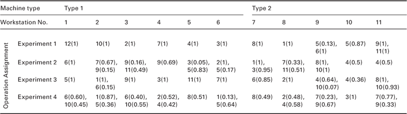
Table 5.12
Optimized production control results of Case 2 of four experiments (without learning effects)
Without learning effects, the operative efficiencies of each operator were unchanged and equal to the operator’s initial efficiencies before production. In other words, the maximum production capacity of production system without learning effects was less than that with learning effects. Even if the production capacity of the FAL decreased, the proposed methodology could still generate effective production control decisions.
In the above experiments, on the basis of different production tasks and production situations, different operation assignments and task proportions were generated. Whichever production tasks and production situations were considered, the optimized production decisions could meet the production objectives, which shows the effectiveness of the proposed decision support system. Moreover, based on the same production task, the generated production decisions with learning effects were different from those without learning effects, owing to the increase of operative efficiencies. Since the production decision without considering learning effect is far from production practice, these effects must be considered in both theory and practice.
The optimized results of this study were obtained based on the following settings:
5.6 Conclusion
This study investigates the production control problem on an FAL, so as to meet the desired cycle time of each order and minimize the total idle time of all workstations on the FAL. The mathematical model of the addressed problem was presented and time-constant learning curve model was adopted to describe the variable operative efficiencies on the FAL. An intelligent decision support system was developed to address the production control problem, in which an RFID-based data capture system was presented to collect the real-time production data from the FAL and a PCDS model was presented to assist in production control decisions on the FAL. In the PCDS model, the mBiGA was used to generate the operation assignment to workstations and task proportions of each shared operation being processed in different workstations. A heuristic operation routing rule was also developed to route the shared operation of each product to an appropriate workstation on a real-time basis. Experimental results were presented to validate the effectiveness of the proposed decision support system. The results confirm that the learning phenomenon should be considered in production control decision-making, because it can result in the increase of operative efficiency and production performance.
This study considers the change of operative efficiency based on the learning curve theory. Since the change of operative efficiency can also be influenced by other factors such as negligence, relearning, and status of machine and operator, future research can focus on the effects of these factors on production control decision-making on the FAL and other production systems.
5.7 Acknowledgement
The authors would like to thank Genexy Company Limited for providing the industrial data and financial support in this research project (Project No. ZW90). Reprinted from Expert Systems with Applications, 36(3), Part 1, Z. X. Guo, W. K. Wong, S. Y. S. Leung, Fan, J. T. and S. F. Chan, Intelligent production control decision support system for flexible assembly lines, 4268–77. Copyright (2009), with permission from Elsevier.
5.8 References
1. Anon. ERP systems can achieve up to 50% higher return on investment when used with RFID mobile data capture systems. Assembly Automation. 2007;27(1):74–75.
2. Arcus AL. COMSOAL: A computer method of sequencing operations for assembly lines. International Journal of Production Research. 1966;4(4):259–277.
3. Badiru A. Computational survey of univariate and multivariate learning-curve models. IEEE Transactions on Engineering Management. 1992;39(2):176–188.
4. Baybars I. A survey of exact algorithms for the simple assembly line balancing problem. Management Science. 1986;32(8):909–932.
5. Beach R, Muhlemann AP, Price DHR, Paterson A, Sharp JA. A review of manufacturing flexibility. European Journal of Operational Research. 2000;122(1):41–57.
6. Becker C, Scholl A. A survey on problems and methods in generalized assembly line balancing. European Journal of Operational Research. 2006;168(3):694–715.
7. Bevis FW. An exploratory study of industrial learning with special reference to work study standards. University of Wales 1970; MSc Thesis.
8. Chan F, Chan H. A comprehensive survey and future trend of simulation study on FMS scheduling. Journal of Intelligent Manufacturing. 2004;15(1):87–102.
9. Charalambous O, Hindi K. A review of artificial intelligence-based job-shop scheduling systems, information and decision technologies. 1991;17(3):189–202.
10. Cheng R, Gen M, Tsujimura Y. A tutorial survey of job-shop scheduling problems using genetic algorithms Part II: Hybrid genetic search strategies. Computers & Industrial Engineering. 1999;37(1–2):51–55.
11. Chong SC, Sivakumar AI, Gay RKL. Simulation-based scheduling for dynamic discrete manufacturing. In: Proceedings of the 2003 Winter Simulation Conference. 2003; New Orleans, LA.
12. Crauwels H, Potts C, Van Oudheusden D, Van Wassenhove L. Branch and bound algorithms for single machine scheduling with batching to minimize the number of late jobs. Journal of Scheduling. 2005;8(2):161–177.
13. Epic Data Inc. RFID Systems. Available from: http://www.epicdata.com/data/rfid-systems.php; 2007; 2007.
14. Framinan J, Gupta J, Leisten R. A review and classification of heuristics for permutation flow-shop scheduling with makespan objective. Journal of the Operational Research Society. 2004;55(12):1243–1255.
15. Gamberini R, Grassi A, Rimini B. A new multi-objective heuristic algorithm for solving the stochastic assembly line re-balancing problem. International Journal of Production Economics. 2006;102(2):226–243.
16. Guo Z, Wong W, Leung S, Fan J, Chan S. A genetic-algorithm-based optimization model for scheduling flexible assembly lines. International Journal of Advanced Manufacturing Technology. 2008;36(1–2):156–168.
17. Gutjahr AL, Nemhauser GL. An algorithm for the line balancing problem. Management Science. 1964;11(2):308–315.
18. Hackett E. Application of a set of learning-curve models to repetitive tasks. Radio and Electronic Engineer. 1983;53(1):25–32.
19. Hitchings B. Dynamic Learning curve models describing the performance of human operators on repetitive industrial tasks. University of Wales 1972; MSc Thesis.
20. Ibraki T, Nakamura Y. A dynamic-programming method for single-machine scheduling. European Journal of Operational Research. 1994;76(1):72–82.
21. Moodie CL, Young HH. A heuristic method of assembly line balancing for assumptions of constant or variable work element times. Journal of Industrial Engineering. 1965;16(1):23–29.
22. Mosheiov G, Sidney J. Scheduling with general job-dependent learning curves. European Journal of Operational Research. 2003;147(3):665–670.
23. MSC Limited. Solution of manufacturing information and management in multi variety and small batch age. Textile & Clothing. 2007;19(1):58–60.
24. Nkasu M, Leung K. A stochastic approach to assembly-line balancing. International Journal of Production Research. 1995;33(4):975–991.
25. Sawik T. Monolithic vs hierarchical balancing and scheduling of a flexible assembly line. European Journal of Operational Research. 2002;143(1):115–124.
26. Scholl A, Becker C. State-of-the-art exact and heuristic solution procedures for simple assembly line balancing. European Journal of Operational Research. 2006;168(3):666–693.
27. Shakhlevich N, Sotskov Y, Werner F. Complexity of mixed shop scheduling problems: A survey. European Journal of Operational Research. 2000;120(2):343–351.
28. Suresh G, Sahu S. Stochastic assembly-line balancing using simulated annealing. International Journal of Production Research. 1994;32(8):1801–1810.
29. Thorndike EL. Animal intelligence: An experimental study of the associative processes in animals. The Psychological Review: Ser Monograph Supplements. 1898;2(8):1–109.
30. Thurstone LL. The learning curve equation. Psychological Monographs. 1919;26(114):51.
31. Wang J, Xia Z. Flow-shop scheduling with a learning effect. Journal of the Operational Research Society. 2005;56(11):1325–1330.
32. Wright T. Factors affecting the cost of airplanes. Journal of Aeronautical Science. 1936;3(4):122–128.