CHAPTER 6
Filters
Introduction
Analogue filter design is an enormous subject, and it is of course quite impossible to cover even its audio aspects in a single chapter. A much, much more detailed account is given in my book The Design of Active Crossovers, which gives practical examples of just about every filter type you can think of. [1] Get the second edition which is much more comprehensive. There are several standard textbooks on filter theory [2] [3] [4], and there would be no point in trying to create another one here. This chapter instead gives information on audio applications not found in the standard textbooks.
Filter design is at the root highly mathematical, and it is no accident that all of the common filter characteristics such as Bessel, Gaussian, Chebyshev, and Legendre are named after mathematicians. A notable exception is the Butterworth characteristic, probably the most popular and useful characteristic of all; Stephen Butterworth was a British engineer. [5] Here I am going to avoid the complexities of pole and zero placement, etc., and concentrate on practical filter designs that can be adapted for different frequencies by simply scaling component values. Most filter textbooks give complicated equations for calculating the amplitude and phase response at any desired frequency. This is less necessary now that access can be assumed to a simulator, which will give all the information you could possibly want, much more quickly and efficiently than wrestling with calculations. Free simulator packages can be downloaded. Filters are widely used in different kinds of audio system, and I make frequent references to them in other chapters.
Filters are either passive or active. Passive or LCR filters use resistors, inductors, and capacitors only. Active filters use resistors, capacitors, and gain elements such as opamps; active filter technology is usually adopted with the specific intent of avoiding inductors and their well-known limitations. Nevertheless, there are some audio applications in which LCR filters are essential.
Passive Filters
Passive filters do not use active electronics, and this is a crucial advantage in some applications. They are not subject to slew-rate limiting, semiconductor non-linearity, or errors due to falling open-loop gain, and this makes them the best technology for roofing filters. A roofing filter is one that stops out-of-band frequencies before they reach the first stage of electronics and so prevents RF demodulation and slew limiting. A classic application is the use in tape machines of parallel LC circuits to keep bias frequencies out of record amplifiers. They are also used as bias traps in multi-track machines, where recording may be happening on one track while the adjacent track is replaying, to keep the bias out of the replay amplifiers. There are more details in Chapter 11 on tape electronics.
Another application is in the measurement of Class-D power amplifiers, which emit copious quantities of RF that will greatly upset audio measuring equipment. The answer, as described by Bruce Hofer [6], is a passive LCR roofing filter. There are many excellent textbooks that describe LCR filter design, such as [2] and [3], and I am not going into it here. Bias traps are relatively easy to design, as all you have to do is get the centre frequency right and have an appropriate Q.
Active Filters
Active filters do not normally use inductors as such, though configurations such as gyrators that explicitly model the action of an inductor are sometimes used. The active element need not be an opamp; the Sallen and Key configuration requires only a voltage follower, which in some cases can be a simple BJT emitter-follower. Opamps are usual nowadays, however. The rest of this chapter deals only with active filters.
Low-Pass Filters
Probably the most common use of low-pass filters is at the output of DACs to remove the high-frequency spurii that remain after oversampling; see Chapter 26 for more on this. They are also used to explicitly define the upper limit of the audio bandwidth in a system at, say, 50 kHz (see the example of a record-cutting amplifier in Chapter 9), though more often this is done by the casual accumulation of a lot of first-order roll-offs in succeeding stages. This is not a duplication of input RF filtering (i.e. roofing filtering), which, as described in Chapter 18 on line inputs, must be passive and positioned before the incoming signals encounter any electronics which can demodulate RF. Low-pass filters are also used in PA systems to protect power amplifiers and loudspeakers against ultrasonic oscillation in the system.
In what might be called the First Age of Vinyl, a fully equipped preamplifier would certainly have a switchable low-pass filter, called, with brutal frankness, the “scratch” filter. This, having a slope of 12 or 18 dB/octave, faster than the tone-control stage and rolling off at a higher frequency around 5–10 kHz, was aimed at suppressing, or at any rate dulling, record surface noise and the inevitable ticks and clicks; see Chapter 9 for much more on this. Interestingly, preamplifiers today, in the Second Age of Vinyl, rarely have this facility, probably because it requires you to face up to the fact that the reproduction of music from mechanical grooves cut into vinyl is really not very satisfactory. Low-pass filters are of course essential to electronic crossovers for loudspeaker systems.
High-Pass Filters
High-pass filters are widely used. Preamplifiers for vinyl disk usage are commonly fitted with subsonic filtering, often below 10 Hz, to keep disturbances due to record warps and ripples from reaching the loudspeakers. Subsonic noise may affect the linearity of the speaker for the worse, as the bass unit is often moved through a substantial part of its mechanical travel; this is particularly true for reflex designs with no cone loading at very low frequencies. If properly designed, this sort of filtering is considered inaudible by most people. In the First Age of Vinyl, preamplifiers sometimes were fitted with a “rumble filter”, which began operations at a higher frequency, typically 35 or 40 Hz, to deal with more severe disk problems and would not be considered inaudible by anyone. Phono subsonic filtering is comprehensively dealt with in Chapter 9 on moving-magnet preamplifiers.
Mixer input channels very often have a switchable high-pass filter at a higher frequency again, usually 100 Hz. This is intended to deal with low-frequency proximity effects with microphones and general environmental rumblings. The slope required to do this effectively is at least 12 dB/octave, putting it outside the capabilities of the EQ section. Some mixer high-pass filters are third-order (18 dB/octave), and fourth-order (24 dB/octave) ones have been used occasionally. Once again, high-pass filters are used in electronic crossovers.
Combined Low-Pass and High-Pass Filters
When both subsonic and ultrasonic filters are required they can sometimes be economically combined into one stage using only one opamp to give audio band definition. Filter combination is usually only practicable when the two filter frequencies are widely separated. There is more on this in Chapter 9 and much more in The Design of Active Crossovers, second edition. [1]
Band-Pass Filters
Band-pass filters are principally used in mixing consoles and stand-alone equalisers (see Chapter 15). The Q required rarely exceeds a value of 5, which can be implemented with relatively simple active filters, such as the multiple-feedback type. Higher Qs or independent control of all the resonance parameters require the use of the more complex biquad or state-variable filters. Band-pass and notch filters are said to be “tuneable” if their centre frequency can be altered relative easily, say by changing only one component value.
Notch Filters
Notch filters are mainly used in equalisers to deal with narrow peaks in the acoustic response of performance spaces, and in some electronic crossovers, for example [7]. They can also be used to remove a single interfering frequency; once a long time ago, I was involved with a product that had a slide-projector in close proximity to a cassette player. Hi-fi was not the aim, but even so, the enormous magnetic field from the projector transformer induced an unacceptable amount of hum into the cassette tape head. Mu-metal only helped a bit, and the fix was a filter that introduced notches at 50 Hz and 150 Hz, working on the “1-band-pass” principle, of which more later.
All-Pass Filters
All-pass filters are so-called because they have a flat frequency response and so pass all frequencies equally. Their point is that they have a phase shift that does vary with frequency, and this is often used for delay correction in electronic crossovers. You may occasionally see a reference to an all-stop filter, which has infinite rejection at all frequencies. This is a filter designer’s joke.
Filter Characteristics
The simple second-order band-pass responses are basically all the same, being completely defined by centre frequency, Q, and gain. High-pass and low-pass filter characteristics are much more variable and are selected as a compromise between the need for a rapid roll-off, flatness in the passband, and a clean transient response. The Butterworth (maximally flat) characteristic is the most popular for many applications. Filters with pass-band ripple, such as the Chebyshev or the Elliptical types, have not found favour for in-band filtering, such as in electronic crossovers, but were once widely used for applications like ninth-order anti-aliasing filters; such filters have mercifully been made obsolete by oversampling. The Bessel characteristic gives a maximally flat group delay (maximally linear phase response) across the passband, and so preserves the waveform of filtered signals, but it has a much slower roll-off than the Butterworth.
Sallen and Key Low-Pass Filters
The Sallen and Key filter configuration was introduced by R. P. Sallen and E. L. Key of the MIT Lincoln Laboratory as long ago as 1955. [8] It became popular because the only active element required is a unity-gain buffer, so in the days before opamps were cheap it could be effectively implemented with a simple emitter-follower or cathode-follower.
Figure 6.1 shows a second-order low-pass Sallen and Key filter with a -3 dB frequency of 624 Hz and a Q of 0.707, together with the pleasingly simple design equations for cutoff (-3 dB) frequency f0 and Q. It was part of a fourth-order Linkwitz-Riley electronic crossover for a three-way loudspeaker. [9] The main difference you will notice from textbook filters is that the resistor values are rather low and the capacitor values correspondingly high. This is an example of low-impedance design, where low resistor values minimise Johnson noise and reduce the effect of the opamp current noise and common-mode distortion. The measured noise output is -117.4 dBu. This is after correction by subtracting the test gear noise floor.
It is important to remember that a Q of 1 does not give the maximally flat Butterworth response; you must use 0.707. Sallen and Key filters with a Q of 0.5 are used in second-order Linkwitz-Riley crossovers, but these are not favoured because the 12 dB/octave roll-off of the high-pass filter is not steep enough to reduce the excursion of a driver when a flat frequency response is obtained. [9]
Sallen and Key low-pass filters have a lurking problem. When implemented with some opamps, the response does not carry on falling forever at the filter slope –instead it reaches a minimum and starts to come back up at 6 dB/octave. This is because the filter action relies on C1 seeing a low impedance to ground, and the impedance of the opamp output rises with frequency due to falling open-loop gain and hence falling negative feedback. When the circuit of Figure 6.1 is built using a TL072, the maximum attenuation is -57 dB at 21 kHz, rising again and flattening out at -15 dB at 5 MHz. This type of filter should not be used to reject frequencies well above the audio band; a low-pass version of the multiple feedback filter is preferred.
Low-pass filters used to define the top limit of the audio bandwidth are typically second-order with roll-off rates of 12 dB/octave; third-order 18 dB/octave filters are rather rarer, probably because there seems to be a mistaken general feeling that phase changes are more audible at the top end of the audio spectrum than the bottom. Either the Butterworth (maximally flat frequency response) or Bessel type (maximally flat group delay) can be used. It is unlikely that there is any real audible difference between the two types of filter in this application, as most of the action occurs above 20 kHz, but using the Bessel alignment does require compromises in the effectiveness of the filtering because of its slow roll-off. I will demonstrate.

The standard Butterworth filter in Figure 6.2a has its -3 dB point set to 50 kHz, and this gives a loss of only 0.08 dB at 20 kHz, so there is minimal intrusion into the audio band; see Figure 6.3. The response is a useful -11.6 dB at 100 kHz and an authoritative -24.9 dB at 200 kHz. C1 is made up of two 2n2 capacitors in parallel.

Figure 6.3 Frequency response of a 50 kHz Butterworth and a 72 kHz Bessel filter, as in Figure 6.2.
| Frequency | Butterworth 50 kHz | Bessel 50 kHz | Bessel 72 kHz | Bessel 100 kHz |
|---|---|---|---|---|
| 20 kHz | –0.08 dB | –0.47 dB | –0.2 dB | –0.1 dB |
| 100 kHz | –11.6 dB | –10.0 dB | –5.6 dB | –3.0 dB |
| 200 kHz | –24.9 dB | –20.9 dB | –14.9 dB | –10.4 dB |
But let us suppose we are concerned about linear phase at high frequencies, and we decide to use a Bessel filter. The only circuit change is that C1 is now 1.335 times as big as C2 instead of 2 times, but the response is very different. If we design for -3 dB at 50 kHz again, we find that the response is –0.47 dB at 20 kHz; a lot worse than 0.08 dB and not exactly a stunning figure for your spec sheet. If we decide we can live with -0.2 dB at 20 kHz, then the Bessel filter has to be designed for -3 dB at 72 kHz; this is the design shown in Figure 6.2b. Due to the inherently slower roll-off, the response is only down to -5.6 dB at 100 kHz and -14.9 dB at 200 kHz, as seen in Figure 6.3; the latter figure is 10 dB worse than for the Butterworth. The measured noise output for both versions is -114.7 dBu using 5532s (corrected for test gear noise).
If we want to keep the 20 kHz loss to 0.1 dB, the Bessel filter has to be designed for -3 dB at 100 kHz, and the response is now only -10.4 dB down at 200 kHz, more than 14 dB less effective than the Butterworth. These results are summarised in Table 6.1
Discussions of filters always remark that the Bessel alignment has a slower roll-off but often fail to emphasise that it is a much slower roll-off. You should think hard before you decide to go for the Bessel option in this sort of application.
It is always worth checking how the input impedance of a filter loads the previous stage. In this case, the input impedance is high in the pass-band, but above the roll-off point it falls until it reaches the value of R1, which here is 1 kΩ. This is because at high frequencies, C1 is not bootstrapped, and the input goes through R1 and C1 to the low-impedance opamp output, which is effectively at ground. Fortunately. this low impedance only occurs at high frequencies, where one hopes the level of the signals to be filtered out will be low.
Another important consideration with low-pass filters is the balance between the R and C values in terms of noise performance. R1 and R2 are in series with the input, and their Johnson noise will be added directly to the signal. The effect of the amplifier noise current flowing in these resistors will also be added in. Here the two 1 kΩ resistors together generate -119.2 dBu of Johnson noise (22 kHz bandwidth, 25°C). The obvious conclusion is that R1 and R2 should be made as low in value as possible without causing excess loading (and 1 kΩ is not a bad compromise) with C1, C2 scaled to maintain the desired roll-off frequency. The need for specific capacitor ratios creates problems, as capacitors are available in a much more limited range of values than resistors, usually the E6 series, running 10, 15, 22, 33, 47, 68. C1 or C2 often has to be made up of two capacitors in parallel.
Full design details of low-pass filters of many types (Butterworth, Bessel, Linear-phase, etc.) up to sixth order are given in The Design of Active Crossovers, second edition. [1]

A variation on the low-pass Sallen and Key that can avoid capacitor ratio difficulties is shown in Figure 6.4. The unity-gain buffer is replaced with a voltage gain stage; the gain set by R3 and R4 must be 1.586 times (+4.00 dB) for a Q of 0.707. This allows C1 and C2 to be the same value. An equal-resistor-value high-pass filter can be made in exactly the same way.
Sallen and Key High-Pass Filters
Figure 6.5 shows a second-order high-pass Sallen and Key filter with a -3 dB frequency of 5115 Hz and a Q of 0.707, with its design equations; this was another part of the electronic crossover. The capacitors are equal, while the resistors must have a ratio of two. The measured noise output of this filter is -115.2 dBu (corrected).

Figure 6.5 The classic second-order high-pass Sallen and Key filter. Cutoff frequency is 5115 Hz. Q= 0.707.
To get a faster roll-off, we can use a third-order filter, which is a first-order filter (i.e. a simple RC time-constant) cascaded with a second-order filter that has a Q of 1.0, causing a response peak. This peak combined with the slow first-order roll-off gives a flat passband and then a steep roll-off. Figure 6.6a shows a third-order high-pass Butterworth filter with a -3 dB frequency of 100 Hz, as might be used at the front end of a mixer channel. It is built the obvious way, with a first-order filter R1, C1 followed by a unity-gain buffer to give low-impedance drive to the following second-order filter. R2 and R3 now have a ratio of 4 to obtain a Q of 1.0. E24 resistor values are shown, and in this case, they give an accurate response.

Figure 6.6 Two third-order Butterworth high-pass filters with a cutoff frequency of 100 Hz.
A more economical way to make a third-order filter is shown in Figure 6.6b, which saves an opamp section. The resistor values shown are the nearest E96 values to the mathematically exact numbers (1× E96 format) and give an extremely accurate response. The nearest E24 values are R1= 2k4, R2= 910 Ω, and R3= 16 kΩ, giving a very small peaking of 0.06 dB at 233 Hz. Errors due to the capacitor tolerances are likely to be larger than this. The distortion performance may not be as good as for Figure 6.6a.
Fourth-order high-pass filters are the steepest in normal use. They are made by cascading two second-order filters with Qs of 0.54 and 1.31. They can also be implemented in one stage as in Figure 6.6b, as can low-pass filters, but the design process is much more complicated, and they may prove to be more sensitive to component tolerances. Ready-made single-stage filter designs up to sixth order can be found in The Design of Active Crossovers, second edition. [1]
Distortion in Sallen and Key Filters
When they have a signal voltage across them, many capacitor types generate distortion. This unwelcome phenomenon is described in Chapter 2. It afflicts not only all electrolytic capacitors but also some types of non-electrolytic ones. If the electrolytics are being used as coupling capacitors, then the cure is simply to make them so large that they have a negligible signal voltage across them at the lowest frequency of interest; less than 80 mVrms is a reasonable criterion. This means they may have to be 10 times the value required for a satisfactory frequency response.
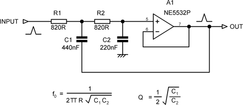
However, because when non-electrolytics are used to set time-constants in filters, they obviously must have substantial signal voltages across them, and this simple fix is not usable. The problem is not a marginal one –the amounts of distortion produced can be surprisingly high. Figure 6.7 shows the frequency response of a conventional second-order Sallen-and-Key high-pass filter as seen in Figure 6.5, with a -3 dB frequency of 520 Hz. C1, C2 were 220 nF 100 V polyester capacitors, with R1= 1 kΩ and R2= 2 kΩ. The opamp was a 5532. The distortion performance is shown by the upper trace in Figure 6.8; above 1 kHz, the distortion comes from the opamp alone and is very low. However, you can see it rising rapidly below 1 kHz as the filter begins to act, and it has reached 0.015% by 100 Hz, completely overshadowing the opamp distortion; it is basically third order. The input level was 10 Vrms, which is about as much as you are likely to encounter in an opamp system. The output from the filter has dropped to -28 dB by 100 Hz, and so the amplitude of the harmonics generated is correspondingly lower, but it is still not a very happy outcome.

Figure 6.7 The frequency response of the second-order 520 Hz high-pass filter.
As explained in Chapter 2, polypropylene capacitors exhibit negligible distortion compared with polyester, and the lower trace in Figure 6.8 shows the improvement on substituting 220 nF 250 V polypropylene capacitors. The THD residual below 500 Hz is now pure noise, and the trace is only rising at 12 dB/octave because circuit noise is constant but the filter output is falling. The important factor is the dielectric, not the voltage rating; 63 V polypropylene capacitors are also free from distortion. The only downside is that polypropylene capacitors are larger for a given CV product and more expensive.
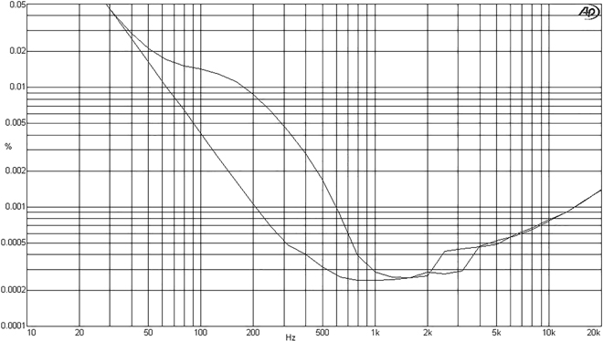
Figure 6.8 THD plot from the second order 520 Hz high-pass filter; input level 10 Vrms. The upper trace shows distortion from polyester capacitors; the lower trace, with polypropylene capacitors, shows noise only below 1 kHz.
Multiple-Feedback Band-Pass Filters
When a band-pass filter of modest Q is required, the multiple-feedback or Rauch type shown in Figure 6.9 has many advantages. The capacitors are equal and so can be made any preferred value. The opamp is working with shunt feedback and so has no common-mode voltage on the inputs, which avoids one source of distortion. It does, however, phase invert, which can be inconvenient.
The filter response is defined by three parameters: the centre frequency f0, the Q, and the passband gain (i.e. the gain at the response peak) A. The filter in Figure 6.8 was designed for f0= 250 Hz, Q=2, and A=1 using the equations given, and the usual awkward resistor values emerged. The resistors in Figure 6.9 are the nearest E96 value (i.e. 1xE96 format), and the simulated results come out as f0 = 251 Hz, Q=1.99, and A=1.0024, which, as they say, is good enough for rock’n roll.

Figure 6.9 A band-pass multiple-feedback filter with f0 = 250 Hz, Q=2 and a gain of 1.
The Q of the filter can be quickly checked from the response curve as Q is equal to the centre frequency divided by the -3 dB bandwidth, i.e. the frequency difference between the two -3 dB points on either side of the peak. This configuration is not suitable for Qs greater than about 10, as the filter characteristics become unduly sensitive to component tolerances. If independent control of f0 and Q are required, the state-variable filter should be used instead.
Similar configurations can be used for low-pass and high-pass filters. The low-pass version does not depend on a low opamp output impedance to maintain stop-band attenuation at high frequencies and avoids the oh-no-it’s-coming-back-up-again behaviour of Sallen and Key low-pass filters.
Notch Filters
There are many ways to dig a deep notch in your frequency response. The width of a notch is described by its Q; exactly as for a resonance peak, the Q is equal to the centre frequency divided by the -3 dB bandwidth, i.e. the frequency difference between the -3 dB points either side of the notch. The Q has no relation to the depth of the notch.
The best-known notch filter is the Twin-T notch network shown in Figure 6.10a, invented in 1934 by Herbert Augustadt. [10] The notch depth is infinite with exactly matched components, but with ordinary ones, it is unlikely to be deeper than 40 dB. It requires ratios of two in component values which do not fit in well with preferred values and when used alone has a Q of only ¼. It is therefore normally used with positive feedback via an opamp buffer A2, as shown. The proportion of feedback K and hence the Q-enhancement is set by R4 and R5, which here give a Q of 1. A great drawback is that the notch frequency can only be altered by changing three components, so it is not considered tuneable.
Another way of making notch filters is the “1-band-pass” principle mentioned earlier. The input goes through a band-pass filter, typically the multiple-feedback type described earlier and is then subtracted from the original signal. The accuracy of the cancellation and hence the notch depth is critically dependent on the mid-band gain of the band-pass filter. Figure 6.10b shows an example that gives a notch at 50 Hz with a Q of 2.85. The subtraction is performed by A2, as the output of the filter is phase inverted. The multiple-feedback filter is designed for unity passband gain, but the use of E24 values as shown means that the actual gain is 0.97, limiting the notch depth to -32 dB. The value of R6 can be tweaked to deepen the notch; the nearest E96 value is 10.2 kΩ, which gives a depth of -45 dB. The final output is inconveniently phase inverted in the passband.
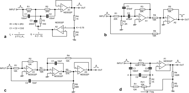
Figure 6.10 Notch filters: a) Twin-T with positive feedback, notch at 795 Hz and a Q of 1; b) “1-band-pass” filter with notch at 50 Hz, Q of 2.85; c) Bainter filter with notch at 700 Hz, Q of 1.29; d) Bridged-differentiator notch filter tuneable 80 to 180 Hz.
A notch filter that deserves to be better known is the Bainter filter [11], [12], shown in Figure 6.10c. It is non-inverting in the passband, and two out of three opamps are working at virtual earth, and will give no trouble with common-mode distortion. An important advantage is that the notch depth does not depend on the matching of components but only on the open-loop gain of the opamps, being roughly proportional to it. With TL072-type opamps, the depth is from -40 to -50 dB. The values shown give a notch at 700 Hz with a Q of 1.29. The design equations can be found in [12].
A property of this filter that does not seem to appear in the textbooks is that if R1 and R4 are altered together, i.e. having the same values, then the notch frequency is tuneable with a good depth maintained, but the Q does change proportionally to frequency. To get a standard notch with equal gain either side of the crevasse, R3 must equal R4. R4 greater than R3 gives a low-pass notch, while R3 greater than R4 gives a high-pass notch; these responses are useful in crossover design. [7] Full design details are given in The Design of Active Crossovers, second edition. [1]
The Bainter filter is usually shown with equal values for C1 and C2. This leads to values for R5 and R6 that are a good deal higher than other circuit resistances, and this will impair the noise performance at very low frequencies. I suggest that C2 is made 10 times C1, i.e. 100 nF, and R5 and R6 are reduced by 10 times to 5.1 kΩ and 6.8 kΩ; the response is unaltered and the Johnson noise much reduced.
But what about a notch filter that can be tuned with one control? Figure 6.10d shows a bridged-differentiator notch filter tuneable from 80 to 180 Hz by RV1. R3 must theoretically be six times the total resistance between A and B, which here is 138 kΩ, but 139 kΩ gives a deeper notch, about -27 dB across the tuning range. The downside is that Q varies with frequency from 3.9 at 80 Hz to 1.4 at 180 Hz.
Another interesting notch filter to look up is the Boctor, which uses only one opamp. [13], [14] Both the biquad and state-variable filters can be configured to give notch outputs.
When simulating notch filters, assessing the notch depth can be tricky. You need a lot of frequency steps to ensure you really have hit bottom with one of them. For example, in one run, 50 steps/decade showed a -20 dB notch, but upping it to 500 steps/decade revealed it was really -31 dB deep. In most cases, having a stupendously deep notch is pointless. If you are trying to remove an unwanted signal, then it only has to alter in frequency by a tiny amount, and you are on the side of the notch rather than the bottom and the attenuation is much reduced. The exception to this is the THD analyser, where a very deep notch (120 dB or more) is needed to reject the fundamental so very low levels of harmonics can be measured. This is achieved by continuously servo-tuning the notch so it is kept exactly on the incoming frequency.
Differential Filters
At first an active filter that is also a differential amplifier, and thereby carries out an accurate subtraction, sounds like a very exotic creature. Actually they are quite common and are normally based on the multiple-feedback filter described here. Their main application is DAC output filtering in CD players and the like; more sophisticated versions are useful for data acquisition in difficult environments. Differential filters are dealt with in the section of Chapter 26 on interfacing with DAC outputs.
References
[1] Self, Douglas The Design of Active Crossovers 2nd edition. Focal Press, 2018
[2] Williams & Taylor Electronic Filter Design Handbook 4th edition. McGraw-Hill, 2006
[3] Van, Valkenburg Analog Filter Design. Holt-Saunders International Editions, 1982
[4] Berlin, H. M. Design of Active Filters with Experiments. Blacksburg, 1978, p 85
[5] Wikipedia http://en.wikipedia.org/wiki/Stephen_Butterworth Accessed Oct 2013
[6] Hofer, Bruce “Switch-mode Amplifier Performance Measurements” Electronics World, Sept 2005, p 30
[7] Hardman, Bill “Precise Active Crossover” Electronics World, Aug 2009, p 652
[8] Sallen & Key “A Practical Method of Designing RC Active Filters” IRE Transactions on Circuit Theory, Vol. 2, No. 1, 1955–3, pp 74–85
[9] Linkwitz, S. “Active Crossover Networks for Non-Coincident Drivers” Journ Aud Eng Soc, Jan/Feb 1976
[10] Augustadt, H. “Electric Filter” US Patent 2,106,785, Feb 1938, assigned to Bell Telephone Labs
[11] Bainter, J. R. “Active Filter Has Stable Notch, and Response Can Be Regulated” Electronics, 2 Oct 1975, pp 115–117
[12] Van, Valkenburg Analog Filter Design, p 346
[13] Boctor, S. A. “Single Amplifier Functionally Tuneable Low-Pass Notch Filter” IEEE Trans Circuits & Systems, Vol. CAS-22, 1975, pp 875–881
[14] Van, Valkenburg Analog Filter Design, Holt-Saunders International Editions 1982, p 349