CHAPTER 9
Moving-Magnet Inputs
Levels and RIAA Equalisation
As stated in the Preface and on the back cover of this book, the publication of Electronics For Vinyl [1] allows the vinyl-oriented material in this book to be drastically cut down so that the space freed can be used for new stuff. All the phono material that was in the second edition of Small Signal Audio Design is in Electronics For Vinyl, plus a great deal more. Therefore, the chapters on moving-magnet inputs have been reduced to one; this cannot and does not give comprehensive coverage of a very big subject, but it will give the most important information, with many pointers to where more (usually much more) can be found in Electronics For Vinyl (EFV). I hope you’ll forgive me for making repeated references to it. I should also say that there are here a few items of information that have been unearthed since EFV was written.
Cartridge Types
This chapter deals with the design of preamplifiers for moving-magnet (MM) cartridge inputs, with their special loading requirements and need for RIAA equalisation. MM cartridges have been for many years less popular than moving-coil (MC) cartridges but now seem to be staging a comeback. However, it would be unusual nowadays to design a phono input that accepted MM inputs only. There are several ways to design a combined MM/MC input, but the approach that gives the best results is to design an MM preamp that incorporates the RIAA equalisation and put a flat-response low-noise head amplifier in front of it to get MC inputs up to MM levels. A large part of this chapter is devoted to the tricky business of RIAA equalisation and so is equally relevant to MC input design; the RIAA just occurs one stage later. Other types of cartridge are the ceramic, (wholly obsolete) strain-gauge cartridges, capacitance pickups, aka “FM pickups”, or electrostatic pickups. The last two are around but are very much in a minority and are not dealt with here.
The Vinyl Medium
The vinyl disc dates back to 1948, when Columbia introduced microgroove 33⅓ rpm LP records. These were followed soon after by microgroove 45 rpm records from RCA Victor. Stereo vinyl did not appear until 1958. The introduction of Varigroove technology, which adjusts groove spacing to suit the amplitude of the groove vibrations, using an extra look-ahead tape head to see what the future holds, allowed increases in groove packing density. This density rarely exceeded 100 grooves per inch in the 78 rpm format, but with Varigroove, 180 to 360 grooves/inch could be used at 33⅓ rpm.
While microgroove technology was unquestionably a considerable improvement on 78 rpm records, any technology that is 60 years old is likely to show definite limitations compared with contemporary standards, and indeed it does. Compared with modern digital formats, vinyl has a restricted dynamic range and poor linearity (especially at the end of a side) and is very vulnerable to permanent and irritating damage in the form of scratches. Even with the greatest care, scratches are likely to be inflicted when the record is removed from its sleeve.
Vinyl discs do not shatter under impact like the 78 shellac discs, but they are subject to warping by heat, improper storage, or poor manufacturing. Possibly the worst feature of vinyl is that the audio signal is degraded every time the disc is played, as the delicate high-frequency groove modulations are worn away by the stylus.
However, for reasons that have very little to do with logic or common sense, vinyl is still very much alive. Even if it is accepted that as a music-delivery medium it is technically as obsolete as wax cylinders, there remain many sizable album collections that it is impractical to replace with CDs and would take an interminable time to transfer to the digital domain. I have one of them. Disc inputs must therefore remain part of the audio designer’s repertoire for the foreseeable future, and the design of the specialised electronics to get the best from the vinyl medium is still very relevant.
If discs are OK, why not cylinders? I thought the release on cylinder of the track “Sewer” in 2010 by the British steampunk band The Men That Will Not Be Blamed For Nothing [2] would be a unique event. It was a very limited edition indeed; only 40 cylinders were produced, and only 30 were put on sale. But not so; in 2013, Ghost wave released a track engraved on a beer bottle; special technology was required to cut the groove into glass. [3] Suzanne Vega has also been recording on cylinders. [4]
Spurious Signals
It is not easy to find dependable statistics on the dynamic range of vinyl, but there seems to be general agreement that it is in the range 50 to 80 dB, the 50 dB coming from the standard-quality discs and the 80 dB representing direct-cut discs produced with quality as the prime aim. My own view is that 80 dB is rather optimistic.
The most audible spurious noise coming from vinyl is that in the mid frequencies, stemming from the inescapable fact that the music is read by a stylus sliding along a groove of finite smoothness. The purely electronic noise will be much lower unless you have a very peculiar (and probably-valve-based) phono amplifier. The Radio Designer’s Handbook says that the groove noise (sometimes called surface noise) of vinyl is 60–62 dB below maximum recorded level, and this will be 20 dB or more above the electronic noise. [5] The best modern reference is Burkhard Vogel’s book, which devotes chapter 11 (no less than 22 pages) to groove noise. [6] He concludes that the best Direct Metal Master mother discs achieve a signal/noise ratio of -72 dB (A-weighted) and 2 dB more are lost in getting to the final pressing. Non-DMM discs will show -64 dB (A-weighted) or worse. This is for brand-new discs and is as good as it gets, because groove noise increases as the record wears with playing. We are therefore looking at (or rather listening to) groove noise which is between -70 and -64 dB below nominal level, not forgetting the A-weighting, and there is nothing that the designer of audio electronics can do about this.
As another data point, a very experienced vinyl enthusiast (60 years plus, going back to shellac) told me that he had never, ever known noise fail to increase when the stylus was lowered onto the run-in groove. [7]
This presents a philosophical conundrum: is it not a waste of time to strive for low electronic noise when the groove noise is much greater and the contribution of the electronic noise negligible? If obtaining a good electronic noise performance was difficult and expensive, this argument would have more force, but it is simply not so. This chapter will show how to get within about 2 dB of the lowest noise physically possible using cheap opamps and a bit of ingenuity. There is also specmanship, of course. The lower the noise specification, the better the sales prospects? One might hope so.
Scratches create clicks that have a large high-frequency content, and it has been shown that they can easily exceed the level of the audio. It is important that such clicks do not cause clipping or slew limiting, as this makes their subjective impact worse.
The signal from a record deck also includes copious amounts of low-frequency noise, which is often called rumble; it is typically below 30 Hz. This can come from several sources:
- Mechanical noise generated by the motor bearings and picked up by the stylus/arm combination. These tend to be at the upper end of the low-frequency domain, extending up to 30 Hz or thereabouts. This is a matter for the mechanical designer of the turntable, as it clearly cannot be filtered out without removing the lower part of the audio spectrum.
- Room vibrations will be picked up if the turntable-and-arm system is not well isolated from the floor. This is a particular problem in older houses where the wooden floors are not built to modern standards of rigidity and have a perceptible bounce to them. Mounting the turntable shelf to the wall usually gives a major improvement. Subsonic filtering is effective in removing room vibration.
- Low-frequency noise from disc imperfections. This can extend as low as 0.55 Hz, the frequency at which a 33⅓ rpm disc rotates on the turntable, and is due to large-scale disc warps. Warping can also produce ripples in the surface, generating spurious subsonic signals up to a few Hertz at surprisingly high levels. These can be further amplified by poorly controlled resonance of the cartridge compliance and the pickup arm mass. When woofer speaker cones can be seen wobbling –and bass reflex designs with no cone loading at very low frequencies are the worst for this –disc warps are usually the cause. Subsonic filtering is again effective in removing this. (As an aside, I have heard it convincingly argued that bass reflex designs have only achieved their current popularity because of the advent of the CD player, with its greater bass signal extension but lack of subsonic output.)
The worst subsonic disturbances are in the region 8–12 Hz, where record warps are accentuated by resonance between the cartridge vertical compliance and the effective arm mass. Reviewing work by Happ and Karlov [8], Bruel and Kjaer [9], Holman [10] [11], Taylor [12], and Hannes Allmaier [13] suggests that in bad cases, the disturbances are only 20–30 dB below maximum signal velocities and that the cart/arm resonance frequency at around 10 Hz should be attenuated by at least 40 dB to reduce its effects below the general level of groove noise. Holman, using a wide variety of cartridge–arm combinations, concluded that to accommodate the very worst cases, a preamplifier should be able to accept not less than 35 mVrms in the 3–4 Hz region. This is a rather demanding requirement, driven by some truly diabolical cartridge–arm setups that accentuated subsonic frequencies by up to 24 dB.
Since the subsonic content generated by room vibrations and disc imperfections tends to cause vertical movements of the stylus, the resulting electrical output will be out of phase in the left and right channels. The use of a central mono subwoofer system that sums the two channels will provide partial cancellation.
Other Vinyl Problems
The reproduction of vinyl involves other difficulties apart from the spurious signals mentioned already:
Distortion is a major problem. It is pretty obvious that the electromechanical processes involved are not going to be as linear as we now expect our electronic circuitry to be. Moving-magnet and moving-coil cartridges add their own distortion, which can reach 1% to 5% at high levels.
Distortion gets worse as the stylus moves from the outside to the inside of the disc. This is called “end-of-side distortion” because it can be painfully obvious in the final track. It occurs because the modulation of the inner grooves is inevitably more compressed than those of the outer tracks due to the constant rotational speed of a turntable. I can well recall buying albums and discovering to my chagrin that a favourite track was the last on a side.
It is a notable limitation of the vinyl process that the geometry of the recording machine and that of the replay turntable do not match. The original recordings are cut on a lathe, where the cutting head moves in a radial straight line across the disc. In contrast, almost all turntables have a pivoting tonearm about 9 inches in length. The pickup head is angled to reduce the mismatch between the recording and replay situations, but this introduces side forces on the stylus and various other problems, increasing the distortion of the playback signal. A recent article in Stereophile [14] shows just how complicated the business of tonearm geometry is. SME produced a 12-inch arm to reduce the angular errors; I have one, and it is a thing of great beauty, but I must admit I have never put it to use.
The vinyl process depends on a stylus faithfully tracking a groove. If the groove modulation is excessive, with respect to the capabilities of the cartridge/arm combination, the stylus loses contact with the groove walls and rattles about a bit. This obviously introduces gross distortion and is also very likely to damage the groove.
A really disabling problem is “wow”, the cyclic pitch change resulting from an off-centre hole. Particularly bad examples of this used to be called “swingers” because they were so eccentric that they could be visibly seen to be rotating off centre. I understand that nowadays the term means something entirely different and relates to an activity that sounds as though it could only distract from critical listening.
Most of the problems that vinyl is heir to are supremely unfixable, but this is an exception; do not underestimate the ingenuity of engineers. In 1983, Nakimichi introduced the extraordinary TX-1000 turntable that measured the disc eccentricity and corrected for it. [15] A secondary arm measured the eccentricity of the run-out groove and used this information to mechanically offset the spindle from the platter bearing axis. This process took 20 seconds, which I imagine could get a bit tedious once the novelty has worn off. This idea deserved to prosper, but CDs were just arriving, and the timing was about as bad as it could be.
Flutter is rapid changes in pitch, rather than the slow ones that constitute wow. You would think that a heavy platter (and some of them are quite ridiculously massive) would be unable to change speed rapidly, and you would be absolutely right. But … the other item in the situation is the cartridge/arm combination, which moves up and down but does not follow surface irregularities because of the resonance between cartridge compliance and arm+cartridge mass. The stylus therefore moves back and forward in the groove, frequency-modulating the signal.
This and the other mechanical issues of turntables and arms are described in an excellent article by Hannes Allmaier [13], who makes the important point that the ear is most sensitive to flutter at around 4 Hz, uncomfortably close to the usual cart/arm resonance region of 8–12 Hz.
Maximum Signal Levels From Vinyl
There are limits to the signal level possible on a vinyl disc and the signal that a cartridge and its associated electronics will be expected to reproduce. The limits may not be precisely defined, but the way they work sets the ways in which maximum levels vary with frequency, and this is of great importance.
There are no variable gain controls on RIAA inputs, because implementing an uneven but very precisely controlled frequency response and a suitably good noise performance are quite hard enough without adding variable gain as a feature. No doubt it could be done, but it would not be easy, there would be issues with channel balance, and the general consensus is that it is not necessary for MM cartridges, which have a range of sensitivities of only 7 dB. If you are using the same stage to RIAA equalise an MC cartridge, the situation is quite different, sensitivities ranging over 36 dB. This is best dealt with by a switched-gain stage rather than fully variable gain.
The overload margin, or headroom, is therefore of considerable importance, and it is very much a case of the more the merrier when it comes to the numbers game of specmanship. The issue is a bit involved, as a situation with frequency-dependant vinyl limitations and frequency-dependant gain is often further complicated by a heavy frequency-dependant load in the shape of the feedback network, which can put its own limit on amplifier output at high frequencies. Let us first look at the limits on the signal levels which stylus-in-vinyl technology can deliver. In the diagrams that follow, the response curves have been simplified to the straight-line asymptotes.
Figure 9.1a shows the physical groove amplitudes that can be put onto a disc. From subsonic up to about 1 kHz, groove amplitude is the constraint. If the sideways excursion is too great, the groove spacing will need to be increased to prevent one groove breaking into another, and playing time will be reduced. Well before actual breakthrough occurs, the cutter can distort the groove it has cut on the previous revolution, leading to “pre-echo” in quiet sections, giving a faint version of the music you are about to hear. Time travel may be fine in science fiction, but it does not enhance the musical experience. The ultimate limit to groove amplitude is set by mechanical stops in the cutter head.

There is an extra limitation on groove amplitude; out-of-phase signals cause vertical motion of the cutter, and if this becomes excessive, it can cause it to cut either too deeply into the disc medium and dig into the aluminium substrate or lose contact with the disc altogether. An excessive vertical component can also upset the playback process, especially when low tracking forces are used; in the worst case, the stylus can be thrown out of the groove completely. To control this problem, the stereo signal is passed through a matrix that isolates the L-R vertical signal, which is then amplitude limited. This potentially reduces the perceived stereo separation at low frequencies, but there appears to be a general consensus that the effect is not audible. The most important factor in controlling out-of-phase signals is the panning of bass instruments (which create the largest cutter amplitudes) to the centre of the stereo stage. This approach is still advantageous with digital media, as it means that there are two channels of power amplification to reproduce the bass information rather than one.
From about 1 kHz up to the ultrasonic regions, the limit is groove velocity rather than amplitude. If the disc cutter head tries to move sideways too quickly compared with its relative forward motion, the back facets of the cutter destroy the groove that has just been cut by its forward edges.
On replay, there is a third restriction: stylus acceleration, or, to put it another way, groove curvature. This limits how well a stylus of a given size and shape can track the groove. Allowing for this at cutting time places an extra limitation on signal level, shown by the dotted line in Figure 9.1a. The severity of this restriction depends on the stylus shape; an old-fashioned spherical type with a tip diameter of 0.7 mil requires a roll-off of maximum levels from 2 kHz, while a (relatively) modern elliptical type with 0.2 mil effective diameter postpones the problem to about 8 kHz. The limit, however, still remains.
Thus disc-cutting and playback technology put at least three limits on the maximum signal level. This is not as bad a problem as it might be, because the distribution of amplitude with frequency for music is not flat with frequency; there is always more energy at LF than HF. This is especially true of the regrettable phenomenon known as rap music. For some reason, there seems to be very little literature on the distribution of musical energy versus frequency, but a very rough rule is that levels can be expected to be fairly constant up to 1 kHz and then fall by something like 10 dB/octave. The end result is that despite the limits on disc levels at HF, it is still possible to apply a considerable amount of HF boost, which, when undone at replay, reduces surface noise problems. At the same time the LF levels are cut to keep groove amplitude under control. Both functions are implemented by applying the inverse of the familiar RIAA replay equalisation at cutting time. More on the limitations affecting vinyl levels can be found on Jim Lesurf’s website. [16]
A reaction to the limitations of the usual 7-inch single was the 12-inch single, which appeared in the mid-1970s, before CDs arrived. The much greater playing area allowed greater groove spacing and higher recording levels. I bought several of these in the 45 rpm format, and I can testify that the greater groove speed gave a much clearer and less distorted high end, definitely superior to 33 rpm LPs.
Since MM input stages not intended for MC use do not normally have gain controls, it is important that they can accept the whole range of input levels that occur. A well-known paper by Tomlinson Holman [17] quotes the worst-case peak voltage from an MM cartridge of 135 mV at 1 kHz given by [18]. This is equivalent to 95 mVrms at 1-kHz. He says, “this is a genuinely worst-case combination which is not expected to be approached typically in practice”.
Shure is a well-known manufacturer of MM cartridges, and its flagship V15 phonograph cartridge series (the 15 in each model name referred to the cartridges’ 15-degree tracking angle) for many years set the standard for low tracking force and high tracking ability. Its development required much research into maximum levels on vinyl. Many other workers also contributed. The results are usually expressed in velocity (cm/s), as this eliminates the effect of cartridge sensitivity. I have boiled down the Shure velocity data into Table 9.1. I have included the acceleration of the stylus tip required for the various frequency/velocity pairs; this is not of direct use, but given that the maximum sustained acceleration the human body can withstand with is around 3 g, it surely makes you think. Since the highest MM cartridge sensitivity for normal use is 1.6 mV per cm/s (see next section), Table 9.1 tells us that we need to be able to handle an MM input of 1.6 ×38 = 61 mVrms. This is not far out of line with the 95 mVrms quoted by Holman, being only 3.8 dB lower.
The website of Jim Lesurf [16] also has many contemporary measurements of maximum groove velocities. The maximum quoted is 39.7 cm/s, which gives 1.6 ×39.7 = 63.5 mVrms. Rooting through the literature, the Pressure Cooker discs by Sheffield Labs were recorded direct to disc and are said to contain velocities up to 40 cm/s, giving us 1.6 ×40 = 64 mVrms. It is reassuring that these maxima do not differ very much. On the other hand, the jazz record Hey! Heard The Herd by Woody Herman (Verve V/V6 8558, 1953) is said to reach a peak velocity of 104 cm/s at 7.25 kHz [18], but this seems out of line with all other data. If it is true, the input level from the most sensitive cartridge would be 1.6 ×105 = 166 mVrms.
| 400 Hz | 500 Hz | 2 kHz | 5 kHz | 8 kHz | 10 kHz | 20 kHz | |
|---|---|---|---|---|---|---|---|
| Velocity cm/s | 26 | 30 | 38 | 35 | 30 | 26 | 10 |
| Acceleration | 66.5 g | 96 g | 487 g | 1120 g | 1535 g | 1665 g | 1281 g |
| Gain dB | Gain times | Max input mVrms | Overload margin dB | 5 mVrms would be raised to: |
|---|---|---|---|---|
| 50 | 316 | 32 mV | 16 dB | 1580 mVrms |
| 45.5 | 188 | 53 mV | 21 dB | 942 mVrms |
| 40 | 100 | 100 mV | 26 dB | 500 mVrms |
| 35 | 56.2 | 178 mV | 31 dB | 281 mVrms |
| 30 | 31.6 | 316 mV | 36 dB | 158 mVrms |
| 25 | 17.8 | 562 mV | 41 dB | 89 mVrms |
| 20 | 10 | 1000 mV | 46 dB | 50 mVrms |
So we may conclude that the greatest input level we are likely to encounter is 64 mVrms, though that 166 mVrms should perhaps not be entirely forgotten.
The maximum input a stage can accept before output clipping is set by its gain and supply rails. If we are using normal opamps powered from ±17 V rails, we can assume an output capability of 10 Vrms. Scaling this down by the gain in each case gives us Table 9.2, which also shows the output level from a nominal 5 Vrms input. You will see shortly why the odd gain value of +45.5 dB was used.
If we want to accept a 64 mVrms input, the gain cannot much exceed +40 dB. In fact, a gain of +43.8 dB will just give clipping for 64 mVrms in. If we want to accept Woody Herman’s 166 mVrms, then the maximum gain is +35.6 dB. I suggest a safety margin of at least 5 dB should be added, so we conclude that 30 dB (1 kHz) is an appropriate gain for an MM input stage; this will accept 316 mVrms from a cartridge before clipping. A recent review of a valve phono stage [19] described an MM input capability of 300 mVrms as “extremely generous”, and I suggest that an input capability of around this figure will render you utterly immune to overload forever and be more than adequate for the highest-quality equipment. The stage output with a nominal 5 mVrms input is only 158 mVrms, which is not enough to operate your average power amplifier, and so there will have to be another amplifying stage after it. This must have switched or variable gain or be preceded by a passive volume control, for otherwise it will clip before the first stage and reduce the overload margin.
While we must have a relatively low gain in the MM stage to give a good maximum signal capability, we do not want it to be too low, or the signal/noise ratio will be unduly degraded as the signal passes through later stages. It is one of the prime rules of audio that you should minimise the possibility of this by getting the signal up to a decent level as soon as possible, but it is common practice and very sensible for the MM output to go through a unity-gain subsonic filter before it receives any further amplification; this is because the subsonic stuff coming from the disc can be at disturbingly high levels.
Moving-Magnet Cartridge Sensitivities
The level reaching the preamplifier is proportional to the cartridge sensitivity. Due to their electromagnetic nature, MM cartridges respond to stylus velocity rather than displacement (the same applies to MC cartridges), so output voltage is usually specified at a nominal velocity of 5 cm/sec. That convention is followed throughout this chapter.
A survey of 72 MM cartridges on the market in 2012 showed that they fall into two groups: what might be called normal hi-fi cartridges (57 of them) and specialised cartridges for DJ use (15 of them). The DJ types have a significantly higher output than the normal cartridges – the Ortofon Q-Bert Concorde produces no less than 11 mV, the highest output I could find. It seems unlikely that the manufacturers are trying to optimise the signal-to-noise ratio in a DJ environment, so I imagine there is some sort of macho “my cartridge has more output than yours” thing going on. Presumably DJ cartridges are also designed to be exceptionally mechanically robust. We will focus here on the normal cartridges, but to accommodate DJ types, all you only really need to do is allow for 6 dB more input level to the preamplifier.

Figure 9.2 Output voltages for 57 MM cartridges at 5 cm/sec, excluding specialised DJ types.
The outputs of the 58 normal cartridges at a velocity of 5 cm/sec are summarised in the histogram of Figure 9.2. The range is 3.0 mV to 8.0 mV, with significant clumps around 4–5 mV and 6.5 mV. If we ignore the single 8.0 mV cartridge, the output range is restricted to 3.0 to 6.5 mV, which is only 6.7 dB. This is a small range compared with the very wide one shown by MC cartridges and makes the design of a purely MM (non-MC) input simpler. There is no need for variable gain, as a 6.7 dB range can be easily accommodated by adjustment of a volume control later in the audio path, without significant noise/headroom compromises.
Overload Margins and Amplifier Limitations
The safety factor between a nominal 5 mVrms input and the clipping point may be described as either the input headroom in mVrms or the “overload margin”, which is the dB ratio between the nominal 5 mVrms input and the maximum input. Table 9.2 shows that an MM stage with a +35 dB gain (1 kHz) gives an output of 280 mV, an input overload level of 178 mVrms, and an overload margin of 31 dB, which might be called very good. A +30 dB (1 kHz) stage gives a nominal 158 mV out, an input overload level of 316 mVrms, and an overload margin of 36 dB, which is definitely excellent, giving 10 dB more headroom.
The maximum input capability of an MM stage is not always defined by simple frequency-independent clipping at its output. Things may be complicated by the stage output capability varying with frequency. An RIAA feedback network, particularly one designed with a relatively low impedance to reduce noise, presents a heavier load as frequency rises because the impedance of the capacitors falls. This HF loading was very often a major cause of distortion and headroom limitation in discrete RIAA stages that had either common-collector or emitter-follower output topologies with highly asymmetrical drive capabilities; for example, an NPN emitter-follower is much better at sourcing current than sinking it. With conventional discrete designs, the 20 kHz output capability, and thus the overload margin, was often reduced by 6 dB or even more. Replacing the emitter resistor of an emitter-follower with a current-source much reduces the problem, and the very slight extra complication of using a push-pull Class-A output structure can bring it down to negligible proportions; for more details, see Chapter 10 on discrete MM input design in Electronics For Vinyl. [1] Earlier opamps such as the TL072 also struggled to drive RIAA networks at HF, as well as giving a very poor noise performance. It was not until the advent of the 5532 opamp, with its excellent load-driving capabilities, that the problem of driving low-impedance RIAA networks was solved; the noise performance was much better, too. However, if a low-impedance HF correction pole (more on this later) is being driven as well, there may still be some slight loss of output capability at 20 kHz.
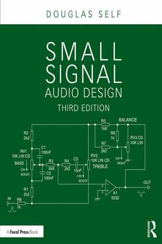
Further headroom restrictions may occur when not all of the RIAA equalisation is implemented in one feedback loop. Putting the IEC Amendment roll-off after the preamplifier stage, as in Figure 9.6, means that very low frequencies are amplified by 3 dB more at 20 Hz than they otherwise would be, and this is then undone by the later roll-off. This sort of audio impropriety always carries a penalty in headroom, as the signal will clip before it is attenuated, and the overload margin at 20 Hz is reduced by 3.0 dB. This effect reduces quickly as frequency increases, being 1.6 dB at 30 Hz and only 1.0 dB at 40 Hz. Whether this loss of overload margin is more important than providing an accurate IEC Amendment response is a judgement call, but in my experience, it creates no trace of any problem in an MM stage with a gain of +30 dB (1 kHz). Passive-equalisation input architectures that put flat amplification before an RIAA stage suffer much more severely from this kind of headroom restriction, and it is quite common to encounter preamplifiers that claim to be high end, with a very high-end price tag but a very low-end overload margin of only 20 to 22 dB. A sad business.
We have to be careful not to compromise the headroom at subsonic frequencies. We saw in the earlier section on spurious signals that Tomlinson Holman concluded that to accommodate the worst of the worst, a preamplifier should be able to accept not less than 35 mVrms in the 3–4 Hz region. If the IEC Amendment is after the preamplifier stage, and C0 is made very large so it has no effect, the RIAA gain in the 2–5 Hz region has flattened out at 19.9 dB, implying that the equivalent overload level at 1 kHz will need to be 346 mVrms. The +30 dB (1 kHz) gain stage of Figure 9.6 has a 1 kHz overload level of 316 mVrms, which is only 0.8 dB below this rather extreme criterion; we are good to go. A +35 dB (1 kHz) gain stage would significantly reduce the safety margin.
At the other end of the audio spectrum, adding an HF correction pole after the preamplifier to correct the RIAA response with low gains also introduces a compromise in the overload margin, though generally a much smaller one. The 30 dB (1 kHz) stage in Figure 9.6 has a mid-band overload margin of 36 dB, which falls to +33 dB at 20 kHz. Only 0.4 dB of this is due to the amplify-then-attenuate action of the HF correction pole, the rest being due to the heavy capacitive loading on A1 of both the main RIAA feedback path and the pole-correcting RC network. This slight compromise could be eliminated by using an opamp structure with greater load-driving capabilities, so long as it retains the low noise of a 5534A.
An attempt has been made to show these extra preamp limitations on output level in Figure 9.1e, and comparing 9.1d, it appears that in practice, they are almost irrelevant because of the falloff in possible input levels at each end of the audio band.
To put things into some sort of perspective, here are the 1 kHz overload margins for a few of my published designs. My first preamplifier, the “Advanced Preamplifier” [20], achieved +39 dB in 1976, partly by using all-discrete design and ±24 V supply rails. A later discrete design in 1979 [21] gave a tour-de-force +47 dB, accepting over 1.1 Vrms at 1 kHz, but I must confess this was showing off a bit and involved some quite complicated discrete circuitry, including the push-pull Class-A output stages mentioned in Self On Audio [22]. Later designs such as the Precision Preamplifier [23] and its linear descendant the Precision Preamplifier ’96 [24] accepted the limitations of opamp output voltage in exchange for much greater convenience in most other directions and still have an excellent overload margin of 36 dB.
Equalisation and Its Discontents
Both moving-magnet and moving-coil cartridges operate by the relative motion of conductors and magnetic field, so the voltage produced is proportional to rate of change of flux. The cartridge is therefore sensitive to groove velocity rather than groove amplitude, and so its sensitivity is expressed as X mV per cm/sec. This velocity sensitivity gives a frequency response rising steadily at 6 dB/octave across the whole audio band for a groove of constant amplitude. Therefore, a maximal signal on the disc, as in Figure 9.1a, would give a cartridge output like Figure 9.1b, which is simply 1a tilted upwards at 6 dB/octave. From here on, the acceleration limits are omitted for greater clarity.
The RIAA replay equalisation curve is shown in Figure 9.1c. It has three corners in its response curve, with frequencies at 50.05 Hz, 500.5 Hz, and 2.122 kHz, which are set by three time-constants of 3180 µsec, 318 µsec, and 75 µsec. The RIAA curve was of USA origin but was adopted internationally with surprising speed, probably because everyone concerned was heartily sick of the ragbag of equalisation curves that existed previously. It became part of the IEC 98 standard, first published in 1964, and is now enshrined in IEC 60098, “Analogue Audio Disk Records and Reproducing Equipment”).
Note the flat shelf between 500 Hz and 2 kHz. It may occur to you that a constant downward slope across the audio band would have been simpler, would have required fewer precision components to accurately replicate, and would have saved us all a lot of trouble with the calculations. But … such a response would require 60 dB more gain at 20 Hz than at 20 kHz, equivalent to 1000 times. The minimum open-loop gain at 20 Hz would have to be 70 dB (3000 times) to allow even a minimal 10 dB of feedback at that frequency, and implementing that with a simple two-transistor preamplifier stage would have been difficult if not impossible. (Must try it sometime.) The 500 Hz–2 kHz shelf in the RIAA curve reduces the 20 Hz–20 kHz gain difference by 12 dB to only 48 dB, making a one-valve or two-transistor preamplifier stage practical. One has to conclude that the people who established the RIAA curve knew what they were doing.
When the RIAA equalisation of Figure 9.1c is applied to the cartridge output of Figure 9.1b, the result looks like Figure 9.1d, with the maximum amplitudes occurring around 1–2 kHz. This is in agreement with Holman’s data. [10]
Figure 9.1e shows some possible output level restrictions that may affect Figure 9.1d. If the IEC Amendment is implemented after the first stage, there is a possibility of overload at low frequencies which does not exist if the amendment is implemented in the feedback loop by restricting C0. At the high end, the output may be limited by problems driving the RIAA feedback network, which falls in impedance as frequency rises. More on this later.
The Unloved IEC Amendment
Figure 9.1c shows in dotted lines an extra response corner at 20.02 Hz, corresponding to a time-constant of 7950 µs. This extra roll-off is called the IEC Amendment, and it was added to what was then IEC 98 in 1976. Its apparent intention was to reduce the subsonic output from the preamplifier, but its introduction is something of a mystery. It was certainly not asked for by either equipment manufacturers or their customers, and it was unpopular with both, with some manufacturers simply refusing to implement it. It still attracts negative comments today. The likeliest explanation seems to be that several noise-reduction systems, for example dbx, were being introduced for use with vinyl at the time, and their operation was badly affected by subsonic disturbances; none of these systems caught on. You would think there must somewhere be an official justification for the Amendment, but if there is, I haven’t found it.
On one hand, critics pointed out that as an anti-rumble measure, it was ineffective, as its slow first-order roll-off meant that the extra attenuation at 13 Hz, a typical cartridge–arm resonance frequency, was a feeble -5.3 dB; however, at 4 Hz, a typical disc warp frequency, it did give a somewhat more useful -14.2 dB, reducing the unwanted frequencies to a quarter of their original amplitude. On the other hand, there were loud complaints that the extra unwanted replay time-constant caused significant frequency response errors at the low end of the audio band, namely –3.0 dB at 20 Hz and –1.0 dB at 40 Hz. Some of the more sophisticated equipment allows the amendment to be switched in or out; a current example is the Audio lab 8000PPA phono preamplifier.
The “Neumann Pole”
The RIAA curve is only defined to 20 kHz but by implication carries on down at 6 dB/octave forever. This implies a recording characteristic rising at 6 dB/octave forever, which could clearly endanger the cutting head if ultrasonic signals were allowed through. From 1995, a belief began to circulate that record lathes incorporated an extra unofficial pole at 3.18μs (50.0 kHz) to limit HF gain. This would cause a loss of 0.17 dB at 10 kHz and 0.64 dB at 20 kHz, and would require compensation if an accurate replay response was to be obtained. The name of Neumann became attached to this concept simply because they are the best-known manufacturers of record lathes.
The main problem with this story is that it is not true. The most popular cutting amplifier is the Neumann SAL 74B, which has no such pole. For protection against ultrasonics and RF, it has instead a rather more effective second-order low-pass filter with a corner frequency of 49.9 kHz and a Q of 0.72 [25], giving a Butterworth (maximally flat) response rolling-off at 12 dB/octave. Combined with the RIAA equalisation, this gives a 6dB/octave roll-off above 50 kHz. The loss from this filter at 20 kHz is less than –0.1 dB, so there is little point in trying to compensate for it, particularly because other cutting amplifiers are unlikely to have identical filters.
MM Amplifier Configurations
There are many ways to make MM input stages, but a fundamental divide is the choice of series or shunt negative feedback. The correct answer is to always use series feedback, as it is about 14 dB quieter; this is because the cartridge loading resistor Rin has a high value and generates a lot of Johnson noise. In the series feedback circuit of Figure 9.3, Rin is in parallel with the cartridge, which shunts away the noise except at high frequencies. In the shunt feedback circuit of Figure 9.4, the input resistor R0 has to be 47 kΩ to load the cartridge correctly, and all its noise goes into the amplifier. The shunt RIAA network has to operate at a correspondingly high impedance and will be noisier. It is a difference that is hard to overlook.
In Figure 9.3, C0 has been given a low value that implements the IEC Amendment. If the amendment is not required, C0 would be of the order of 220 μF.
The only drawback of the series-feedback configuration is that its gain cannot fall below unity. The RIAA curve is only defined to 20 kHz, but as noted, by implication, it carries on down at 6 dB/octave forever. If the stage has a gain of less than +35 dB (1 kHz), this causes the response to level out and causes RIAA errors in the top octaves. This can be completely cured by adding an HF correction RC time-constant just after the amplifier. See Figure 9.6.

Figure 9.3 Series-feedback RIAA equalisation Configuration A, IEC Amendment implemented by C0. Component values for 35.0 dB gain (1 kHz). Maximum input 178 mVrms (1 kHz). RIAA accuracy is within ±0.1 dB from 20 Hz to 20 kHz, without using an HF correction pole.

The shunt-feedback configuration has occasionally been advocated because it avoids the unity-gain problem, but it has the crippling disadvantage that with a real cartridge load, with its substantial inductance, it is about 14 dB noisier than the series configuration. [26] This is because the Johnson noise from R0 is not shunted away at LF by the cartridge inductance and because the current noise of A1 sees R0 + the cartridge inductance instead of R0 in shunt with the cartridge inductance. A great deal of grievous twaddle has been talked about RIAA equalisation and transient response in perverse attempts to render the shunt RIAA configuration acceptable despite its serious noise disadvantage.
Shunt feedback eliminates any possibility of common-mode distortion, but then at the signal levels we are dealing with, that is not a problem, at least with bipolar input opamps. A further disadvantage is that a shunt-feedback RIAA stage gives a phase inversion that can be highly inconvenient if you are concerned to preserve absolute phase.
Remarkably, someone called Mohr managed to get a US patent for a variation of this idea in which the cartridge load is effectively a short circuit. [27] The patent is considered to be of no value. The fascinating thing about it is that while noise is barely mentioned, a reference is given to [26] as given earlier; this is HP Walker’s famous article on noise in which the inherent inferiority of the shunt version was clearly demonstrated. Presumably Mohr never actually read it.
Opamp MM Input Stages
Satisfactory discrete MM preamplifier circuitry is not that straightforward to design, and there is a lot to be said for using a good opamp, which, if well chosen, will have more than enough open-loop gain to implement the RIAA bass boost accurately and without introducing detectable distortion at normal operating levels. The 5534/5532 opamps have input noise parameters that are well suited to moving-magnet (MM) cartridges –better so than any other opamp? They also have good low-distortion load-driving capability so the RIAA network impedances can be kept low.
Having digested this chapter so far, we are in a position to summarise the requirements for a good RIAA preamplifier. These are:
- Use a series feedback RIAA network, as shunt feedback is approximately 14 dB noisier.
- Correct gain at 1 kHz. This sounds elementary, but getting the RIAA network right is not a negligible task.
- RIAA accuracy. My 1983 preamplifier was designed for +/-0.2 dB accuracy from 20–20 kHz, the limit of the test gear I had at the time. This was tightened to +/-0.05 dB without using rare parts in my 1996 preamplifier.
- Use obtainable components. Resistors will often be from the E24 series, though E96 is much more available than it used to be. Capacitors will probably be from the E6 or E12 series, so intermediate values must be made by series or parallel combinations.
- R0 should be as low as its Johnson noise is effectively in series with the input signal. This is particularly important when the MM preamplifier is fed from a low impedance, which typically occurs when it is providing RIAA equalisation for the output of an MC preamplifier. With input direct from an MM cartridge with its high inductance, the effect of R0 on noise is weak.
- The feedback RIAA network impedance to be driven must be suited to the opamp to prevent increased distortion or a limited output swing, especially at HF.
- The resistive path through the feedback arm should ideally have the same DC resistance as input bias resistor Rin to minimise offsets at A1 output. This is a bit of a minor point, as the offset would have to be quite large to significantly affect the output voltage swing (DC blocking is assumed). Very often it is not possible to meet this constraint as well as other more important requirements.
Calculating the RIAA Equalisation Components
Calculating the values required for series feedback configuration is not straightforward. You absolutely cannot take Figure 9.3 and calculate the time-constants of R2, C2 and R3, C3 as if they were independent of each other; the answers will be wrong. Empirical approaches (cut-and-try) are possible if no great accuracy is required, but attempting to reach even ±0.2 dB by this route is tedious, frustrating, and generally bad for your mental health.
The definitive paper on this subject is by Stanley Lipshitz. [28] This heroic work covers both series and shunt configurations and much more besides, including the effects of low open-loop gain. It is relatively straightforward to build a spreadsheet using the Lipshitz equations that allows extremely accurate RIAA networks to be designed in a second or two; the greatest difficulty is that some of the equations are long and complicated –we’re talking real turn-the-paper-sideways algebra here –- and some very careful typing is required.
Exact RIAA equalisation cannot be achieved with preferred component values, and that extends to E24 resistors. If you see any single-stage RIAA preamp where the equalisation is achieved by two E24 resistors and two capacitors in the same feedback loop, you can be sure it is not very accurate.
My spreadsheet model takes the desired gain at 1 kHz and the value of R0, which sets the overall impedance level of the RIAA network. In my preamplifier designs, the IEC Amendment is definitely not implemented by restricting the value of C0; this component is made large enough to have no significant effect in the audio band, and the amendment roll-off is realised in the next stage.
Implementing RIAA Equalisation
It can be firmly stated from the start that the best way to implement RIAA equalisation is the traditional series-feedback method. So-called passive (usually only semi-passive) RIAA configurations suffer from serious compromises on noise and headroom. For completeness, they are dealt with towards the end of this chapter.
There are several different ways to arrange the resistors and capacitors in an RIAA network, all of which give identically exact equalisation when the correct component values are used. Figure 9.3 shows a series-feedback MM preamp built with what I call RIAA Configuration A, which has the advantage that it makes the RIAA calculations somewhat easier but otherwise is not the best; there will be much more on this topic later. Don’t start building it until you’ve read the rest of this chapter; it gives an accurate RIAA response but is not otherwise optimised, as it attempts to represent a “typical” design. We will optimise it later; we will lower the gain and reduce the value of R0 to reduce its Johnson noise contribution and the effect of opamp current noise flowing in it. Also note that details that are essential for practical use, like input DC-blocking capacitors, DC drain resistors, and EMC/cartridge-loading capacitors, have been omitted to keep things simple; often the 47 kΩ input loading resistor is omitted as well. The addition of these components is fully described in the section on practical designs at the end of this chapter.
This stage is designed for a gain of 35.0 dB at 1 kHz, which means a maximum input of 178 mV at the same frequency. With a nominal 5 mVrms input at 1 kHz, the output is 280 mV. The RIAA accuracy is within ±0.1 dB from 20 Hz to 20 kHz, and the IEC Amendment is implemented by making C0 a mere 7.96 μF. You will note with apprehension that only one of the components, R0, is a standard value, and that is because it was used as the input to the RIAA design calculations that defined the overall RIAA network impedance. This is always the case for accurate RIAA networks. Here, even if we assume that capacitors of the exact value could be obtained and we use the nearest E96 resistor values, systematic errors of up to 0.06 dB will be introduced. Not a long way adrift, it’s true, but if we are aiming for an accuracy of ±0.1 dB, it’s not a good start. If E24 resistors are the best available, the errors grow to a maximum of 0.12 dB, and don’t forget that we have not considered tolerances –we are assuming the values are exact. If we resort to the nearest E12 value (which really shouldn’t be necessary these days), then the errors exceed 0.7 dB at the HF end. And what about those capacitors?
The answer is that by using multiple components in parallel or series, we can get pretty much what value we like, and it is perhaps surprising that this approach is not adopted more often. The reason is probably cost –a couple of extra resistors are no big deal, but extra capacitors make more of an impact on the costing sheet. The use of multiple components also improves the accuracy of the total value, as described in Chapter 2. More on this important topic later in this chapter.
While the RIAA equalisation curve is not specified above 20 kHz, the implication is clear that it will go on falling indefinitely at 6 dB/octave. A series feedback stage cannot have a gain of less than unity, so at some point, the curve will begin to level out and eventually become flat at unity gain; in other words, there is a zero in the response.
Figure 9.5 shows the frequency response of the circuit in Figure 9.3, with its associated time-constants. T3, T4, and T5 are the time-constants that the define the basic RIAA curve, while f3, f4, and f5 are the equivalent frequencies. This is the naming convention used by Stanley Lipshitz in his landmark paper [28], and it is used throughout this book. Likewise, T2 is the extra time-constant for the IEC Amendment, and T1 shows where its effect ceases at very low frequencies when the gain is approaching unity at the low frequency end due to C0. At the high end, the final zero is at frequency f6, with associated time-constant T6, and because the gain was chosen to be +35 dB at 1 kHz, it is quite a long way from 20 kHz and has very little effect at this frequency, giving an excess gain of only 0.10 dB. This error quickly dies away to nothing as frequency falls below 20 kHz.
As noted, the series-feedback RIAA configuration has what might be called the unity-gain problem. If the gain of the stage is set lower than +35 dB to increase the input overload margin, the 6dB/octave fall tends to level out at unity early enough to cause significant errors in the audio band. Adding an HF correction pole (i.e. low-pass time-constant) just after the input stage makes the simulated and measured frequency response exactly correct. It is NOT a question of bodging the response to make it roughly right. If the correction pole frequency is correctly chosen, the roll-off cancels exactly with the “roll-up” of the final zero at f6.
An HF correction pole is demonstrated in Figure 9.6, where several important changes have been made compared with Figure 9.3. The overall impedance of the RIAA network has been reduced by making R0 220 Ω, to reduce Johnson noise from the resistors; we still end up with some very awkward values.

The IEC Amendment is no longer implemented in this stage; if it was, then the correct value of C0 would be 36.18 μF, and instead it has been made 220 μF so that its associated -3 dB roll-off does not occur until 3.29 Hz. Even this wide spacing introduces an unwanted 0.1 dB loss at 20 Hz, and perfectionists will want to use 470 μF here, which reduces the error to 0.06 dB.
Most importantly, the gain has been reduced to +30 dB at 1 kHz to get more overload margin. With a nominal 5 mVrms input at 1 kHz, the output will be 158 mV. The result is that the flattening-out frequency f6 in Figure 9.3 is now at 66.4 kHz, much closer in, and it introduces an excess gain at 20 kHz of 0.38 dB, which is too much to ignore if you are aiming to make high-class gear. The HF correction pole R4, C4 is therefore added, which solves the problem completely. Since there are only two components and no interaction with other parts of the circuit, we have complete freedom in choosing C4, so we use a standard E3 value and then get the pole frequency exactly right by using two resistors in series for R4–470 Ω and 68 Ω. Since these components are only doing a little fine tuning at the top of the frequency range, the tolerance requirements are somewhat relaxed compared with the main RIAA network. The design considerations are a) that the resistive section R4 should be as low as possible in value to minimise Johnson noise and on the other hand b) that the shunt capacitor C4 should not be large enough to load the opamp output excessively at 20 kHz. At this level of accuracy, even the finite gain open-loop gain of even a 5534 at HF has a slight effect, and the frequency of the HF pole has been trimmed to compensate for this.
Implementing the IEC Amendment
The unloved IEC Amendment was almost certainly intended to be implemented by restricting the value of the capacitor at the bottom of a series feedback arm, i.e. C0 in Figures 9.3 and 9.6. While electrolytic capacitors nowadays (2013) have relatively tight tolerances of ±20%, in the 1970s, you would be more likely to encounter -20% +50%, the asymmetry reflecting the assumption that electrolytics would be used for non-critical coupling or decoupling purposes where too little capacitance might cause a problem, but more than expected would be fine. This wide tolerance meant that there could be significant errors in the LF response due to C0. Figure 9.7 shows the effect of a ±20% C0 tolerance on the RIAA response of a preamplifier similar to Figure 9.6, with a gain of +30 dB (1 kHz) and C0 = 36.13 uF. The gain will be +0.7 dB up at 20 Hz for a +20% C0 and -1.1 dB down at 20 Hz for a -20% C0. The effect of C0 is negligible above 100 Hz, but this is clearly not a good way to make accurate RIAA networks.
To get RIAA precision, it is necessary to implement the IEC Amendment separately with a non-electrolytic capacitor, which can have a tolerance of ±1% if necessary. In several of my designs, the IEC Amendment has been integrated into the response of the subsonic filter that immediately follows the RIAA preamplifier; this gives economy of components but means that it is not practicable to make it switchable in and out. Unless buffering is provided, the series resistance in the HF correction network can interfere with the subsonic filter action, causing an early roll-off that degrades RIAA accuracy in the 20–100 Hz region.
The best solution is a passive CR high-pass network after the preamplifier stage. We make C0 large to minimise its effect and add a separate 7950 µs time-constant after the preamplifier, as shown in Figure 9.6, where R3 and C3 give the required -3 dB roll-off at 20.02 Hz.
Another problem with the “small C0” method of IEC Amendment is the non-linearity of electrolytic capacitors when they are asked to form part of a time-constant. This is described in detail in Chapter 2. Since the MM preamps of the seventies tended to have poor linearity at LF anyway, because the need for bass boost meant a reduction in the LF negative feedback factor, introducing another potential source of distortion was not exactly an inspired move; on the other hand, the signal levels are low. There is no doubt that even a simple second-order subsonic filter, switchable in and out, is a better approach to controlling subsonic disturbances. If a Butterworth (maximally flat) alignment was used, with a –3 dB point at 20 Hz, this would only attenuate by 0.3 dB at 40 Hz but would give a more useful -8.2 dB at 13 Hz and a thoroughly effective -28 dB at 4 Hz. Not all commentators are convinced that the more rapid LF phase changes that result are wholly inaudible, but they are; you cannot hear phase, as explained in Chapter 1. Subsonic filters are examined more closely at the end of this chapter.

Figure 9.7 The effect of a ±20% tolerance for C0 when it is used to implement the IEC Amendment.
RIAA Series-Feedback Network Configurations
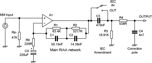
So far, we have only looked at one way to construct the RIAA feedback network. There are other ways, because it does not matter how the time-constants are implemented, just that they are correct. There are four possible configurations described by Lipshitz in his classic paper. [28] These are shown in Figure 9.8; the same identifying letters have been used. Note that the component values have been scaled compared with the original paper so that all versions have a closed-loop gain of +45.5 dB at 1 kHz, and all have R0 = 220Ω to aid comparison.
All four versions are accurate to within ±0.1 dB when implemented with a 5534 opamp, but in the case of Figure 9.8a, the error is getting close to -0.1 dB at 20 Hz due to the relatively high closed-loop gain and the finite open-loop gain of the 5534. All have RIAA networks at a relatively high impedance. They all have relatively high gain and therefore a low maximum input. The notation R0, C0, R1, C1, R2, C2 is as used by Lipshitz; C1 is always the larger of the two. In each case, the IEC Amendment is implemented by the value of C0.

So there are the four configurations; is there anything to choose between them? Yes indeed. First, each configuration in Figure 9.8 contains two capacitors, a large C1 and a small C2. If they are close tolerance (to get accurate RIAA) and non-polyester (to prevent capacitor distortion), then they will be expensive, so if there is a configuration that makes the large capacitor smaller, even if it is at the expense of making the small capacitor bigger, it is well worth pursuing. The large capacitor C1 is probably the most expensive component in the RIAA MM amplifier by a large margin.
Configuration A (which I have been using for years) makes the least efficient use of its capacitors, since they are effectively in series, reducing the effective value of both of them. Configuration C has its capacitors more in parallel, so to speak, and has the smallest capacitors for both C1 and C2. Configurations B and D have intermediate values for C1, but of the two, D has a significantly smaller C2. Configuration C is the optimal solution in terms of capacitor size and hence cost. To design it accurately for gains other than +45.5 dB (1 kHz) meant building a software tool for it from the Lipshitz equations for Configuration C. This I duly did, though just as anticipated, it was somewhat more difficult than it had been for Configuration A.
The scaling process slightly reduced the RIAA accuracy, so Configuration A was recalculated from scratch using the Lipshitz equations; see Figure 9.9.
While Configuration C in Figures 9.8 and 9.9 has come out as the most economical, our work here is not done. It will not have escaped you that a gain as high as +45.5 dB at 1 kHz is not going to give a great overload margin; it has only been used so far because it was the gain adopted in the Lipshitz paper. If we assume our opamp can provide 10 Vrms out, then the maximum input at 1 kHz is only 53 mVrms, which is mediocre at best. The gain of an MM input stage should not, in my opinion, much exceed 30 dB at 1 kHz. (See the earlier example in Figure 9.6.)
My Precision Preamplifier design [23] has an MM stage gain of +29 dB at 1 kHz, allowing a maximum input of 354 mVrms (1 kHz). The more recent Elektor Preamplifier 2012 [29] has an MM stage gain of +30 dB (1 kHz), allowing a maximum input of 316 mVrms; it is followed by a flat switched-gain stage which allows for the large range in MC cartridge sensitivity.
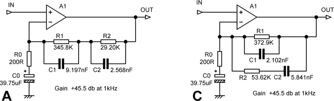
I used the new software tool for Configuration C to design the MM input stage in Figure 9.10, which has a gain of +30 dB (1 kHz). This design has an RIAA response, including the IEC Amendment, that is accurate to within ±0.01 dB from 20 Hz to 20 kHz. (It is assumed C0 is accurate.) The relatively low gain means that an HF correction pole is required to maintain accuracy at the top of the audio band, and this is implemented by R3 and C3. Without this pole, the response is 0.1 dB high at 10 kHz and 0.37 dB high at 20 kHz. R3 is a non-preferred value, as we have used the E6 value of 2n2 for capacitor C3.
In Figure 9.10 and in the examples that follow, I have implemented the IEC Amendment by using the appropriate value for C0 rather than by adding an extra time-constant after the amplifier as in Figure 9.6. We noted that using C0 is not the best method, but I have stuck with it here, as it is instructive how the correct value of C0 changes as other alterations are made to the RIAA network. In many cases, the IEC Amendment is just not wanted, and C0 will be 220 μF or 470 μF. It is assumed there will be a proper subsonic filter later in the signal path.
Figure 9.10 Configuration C with values calculated from the Lipshitz equations to give +30.0 dB gain at 1 kHz and an accurate RIAA response within ±0.01 dB; the lower gain now requires HF correction pole R3, C3 to maintain accuracy at the top of the audio band.
RIAA Optimisation: C1 as a Single E6 Capacitor, 2xE24
Looking at Figure 9.10, a further stage of optimisation is possible after choosing the best RIAA configuration. There is nothing magical about the value of R0 at 200 Ω (apart from the bare fact that it’s an E24 value); it just needs to be suitably low for a good noise performance so it can be manipulated to make at least one of the capacitor values more convenient, the larger one being the obvious candidate. Compared with the potential savings on expensive capacitors here, the cost of a non-preferred value for R0 is negligible. It is immediately clear that C1, at 34.9 nF, is close to 33 nF. If we twiddle the new software tool for Configuration C so that C1 is exactly 33 nF, we get the arrangement in Figure 9.11. R0 has only increased by 6%, and so the effect on the noise performance will be quite negligible. All the values in the RIAA feedback network have likewise altered by about 6%, including C0, but the HF correction pole is unchanged; we would only need to alter it if we altered the gain. The RIAA accuracy of Figure 9.11 is still well within ±0.01 dB from 20 Hz to 20 kHz when implemented with a 5534.
The circuit of Figure 9.11 has two preferred-value capacitors, C1 and C3, but that is the most we can manage. All the other values are, as expected, thoroughly awkward. The resistor values can be tackled by using the E96 series, but it may mean keeping an awful lot of values in stock. There are better ways…

In Chapter 2, I describe how to make up arbitrary resistor values by paralleling two or more resistors and how the optimal way to do this is with resistors of as nearly equal values as you can manage. If the values are equal, then the tolerance errors partly cancel, and the accuracy of the combination is √2 times better than the individual resistors. The resistors are assumed to be E24, and the parallel pairs were selected using a specially written software tool. The three-part combination for C2, which I have assumed restricted to E6 values, works out very nicely, with only three components getting us very close to the exact value we want. Table 9.3 gives the component combinations, and Figure 9.12 shows the practical circuit that results.
The criterion used when selecting the parallel resistor pairs was that the error in the nominal value should be less than half of the component tolerance, assumed to be ±1%. In Table 9.3, R2 only just squeaks in, but its near-equal values will give almost all of the √2 (=0.707) improvement possible. Remember that in Table 9.3, we are dealing here with nominal values, and the percentage error in the nominal value shown in the “Error” column has nothing to do with the resistor tolerances. The effective tolerance of the combination for each component is shown in the rightmost column, and all are an improvement on 1% except for C1, as it is a single component.
No attempt has been made here to deal with the non-standard value for C0. In practice, C0 will be a large value such as 220 μF, so its wide tolerance will have no significant effect on RIAA accuracy. The IEC Amendment will be implemented (if at all) by a later time-constant using a non-electrolytic, as shown earlier in Figure 9.6.
| Component | Desired value | Actual value | Parallel part A | Parallel part B | Parallel part C | Nominal error | Effective tolerance |
|---|---|---|---|---|---|---|---|
| R0 | 211.74 Ω | 211.03 Ω | 360 Ω | 510 Ω | – | –0.33% | 0.72% |
| R1 | 66.18 kΩ | 65.982 kΩ | 91 kΩ | 240 kΩ | – | –0.30% | 0.78% |
| C1 | 33 nF | 33 nF | 33 nF | – | – | 0% | 1.00% |
| R2 | 9.432 kΩ | 9.474 kΩ | 18 kΩ | 20 kΩ | – | +0.44% | 0.71% |
| C2 | 11.612 nF | 11.60 nF | 4n7 | 4n7 | 2n2 | –0.10% | 0.60% |
| R3 | 1089.2 Ω | 1090.9Ω | 2 kΩ | 2.4 kΩ | – | +0.16% | 0.71% |
RIAA Optimisation: C1 as 3 x 10 nF Capacitors, 2xE24
We have just modified the RIAA network so that the major capacitor C1 is a single preferred value. The optimisation of the RIAA component values can be tackled in another way, however; much depends on component availability. In many polystyrene capacitor ranges, 10 nF is the highest value that can be obtained with a tolerance of 1%; in other cases, the price goes up rather faster than proportionally above 10 nF. Paralleling several 10 nF polystyrene capacitors is much more cost effective than using a single precision polypropylene part.
| Component | Desired value | Actual value | Parallel part A | Parallel part B | Parallel part C | Nominal error | Effective tolerance |
|---|---|---|---|---|---|---|---|
| R0 | 232.9 Ω | 233.3 Ω | 430 Ω | 510 Ω | – | –0.17% | 0.71% |
| R1 | 72.64 kΩ | 72.64 kΩ | 91 kΩ | 360 kΩ | – | –0.002% | 0.82% |
| C1 | 30 nF | 30 nF | 10 nF | 10 nF | 10 nF | 0% | 0.58% |
| R2 | 10.375 kΩ | 10.359 kΩ | 13 kΩ | 51 kΩ | – | –0.15% | 0.82% |
| C2 | 10.557 nF | 10.52 nF | 4n7 | 4n7 | 1 nF + 120 pF | –0.34% | 0.64% |
| R3 | 1089.2 Ω | 1090.9Ω | 2 kΩ | 2.4 kΩ | – | +0.16% | 0.71% |
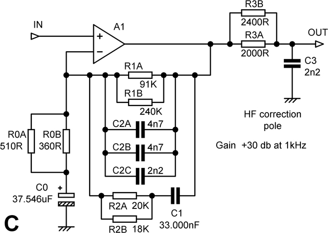
To use this method, we need to redesign the circuit of Figure 9.12 so that C1 is either exactly 30 nF or exactly 40 nF. (There is a practical design using Configuration A with 5 x 10 nF = 50 nF at the end of this chapter, underlining the fact that Configuration A makes less efficient use of its capacitance.) The 40 nF version costs more than the 30 nF version but gives a total capacitance that is twice as accurate as one capacitor (because √4 = 2), while the 30 nF version only improves accuracy by √3 (= 1.73) times. Using 40 nF gives somewhat lower general impedance for the RIAA network, but this will only reduce noise very slightly. Figure 9.13 and Table 9.4 show the result for C1 = 30 nF, and Figure 9.14 and Table 9.5 show the result for C1 = 40 nF. In both cases, the resistors are made up of 2xE24 pairs. Since the gain is unchanged the values for the HF correction pole R3, C3 are also unchanged in each case.
In the +30 dB case, we have been unlucky with the value of C2, which needs to be trimmed with a 120 pF capacitor to meet the criterion that the error in the nominal value will not exceed half the component tolerance. This configuration has been built with 1% capacitors and thoroughly measured, and it works exactly as it should. It gave a parts-cost saving of about £2 on the product concerned. That feeds through to a significant reduction in the retail price.
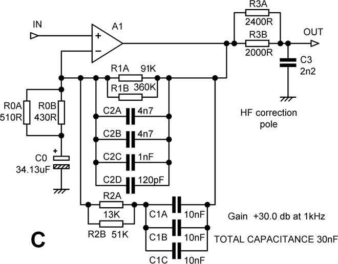
RIAA Optimisation: C1 as 4 x 10 nF Capacitors, 2xE24
The same process can be applied to the C1 = 4 x 10 nF version, giving the results in Table 9.5 and Figure 9.14.
This time, we are much luckier with the value of C2; three 4n7 capacitors in parallel give almost exactly the required value and a healthy improvement in the effective tolerance 0.58%. On the other hand, we are very unlucky with R0, where 180 Ω in parallel with 6.2 kΩ is the most “equal-value” solution that falls within our error criterion, and there is negligible improvement in the effective tolerance.
RIAA Optimisation: The Willmann Tables
The 2xE24 examples given in the previous section use two resistors in parallel, and the relatively small number of combinations available means that the nominal value is not always as accurate as we would like; for example, the 0.44% error in Table 9.3, which only just meets the rule that “The nominal value of the combination shall not differ from the desired value by more than half the component tolerance”. For the usual 1% parts, this means within ±0.5%, and once that is achieved, we can pursue the goal of keeping the values as near equal as possible. Keep in mind that ±0.5% is the error in the nominal value, and the component tolerance, or the effective component tolerance when two or more resistors are combined, is another thing entirely and a source of additional error. It is usually best to use parallel rather than series combinations of resistors, because it makes the connections on a PCB simpler and more compact.
| Component | Desired value | Actual value | Parallel part A | Parallel part B | Parallel part C | Parallel part D | Nominal error | Effective tolerance |
|---|---|---|---|---|---|---|---|---|
| R0 | 174.7 Ω | 174.9 Ω | 180 Ω | 6.2 kΩ | – | – | +0.13% | 0.97% |
| R1 | 54.65 kΩ | 54.54 kΩ | 100 kΩ | 120 kΩ | – | – | +0.19% | 0.71% |
| C1 | 40 nF | 40 nF | 10 nF | 10 nF | 10 nF | 10 nF | 0% | 0.50% |
| R2 | 7.821 kΩ | 7.765 kΩ | 12 kΩ | 22 kΩ | – | – | –0.22% | 0.74% |
| C2 | 14.074 nF | 14.1 nF | 4n7 | 4n7 | 4n7 | – | +0.18% | 0.58% |
| R3 | 1089.2 Ω | 1090.9Ω | 2 kΩ | 2.4 kΩ | – | – | +0.16% | 0.71% |
The relatively small number of combinations of E24 resistor values also means that it is difficult to pursue good nominal accuracy and effective tolerance reduction at the same time. This can be addressed by instead using three E24 resistors in parallel, as noted in Chapter 2. I call this the 3xE24 format. Given the cheapness of resistors, the economic penalties of using three rather than two to approach the desired value very closely are small, and the extra PCB area required is modest. However, the design process is significantly harder.
The process is made simple by using one of the resistor tables created by Gert Willmann. There are many versions, but the one I used lists in text format all the three-resistor E24 parallel combinations and their combined value. It covers only one decade, which is all you need, but is naturally still a very long list, running to 30,600 entries. The complete Willmann Tables cover a wide range of resistor series, parallel/series connections, and so on. Gert Willmann has very kindly made the tables freely available, and the complete collection can be downloaded free of charge from my website at [30].
RIAA Optimisation: C1 as 3 x 10 nF Capacitors, 3xE24
I first applied the Willmann Table process to Figure 9.11, which has +30 dB gain at 1 kHz and C1 set to exactly 33 nF. I started with R0, which has a desired value of 211.74Ω. The appropriate Willmann table was read into a text editor, and using the search function to find “211.74” takes us straight to an entry at line 9763 for 211.74396741Ω, made up of 270Ω, 1100 Ω, and 9100Ω in parallel. This nominal value is more than accurate enough, but since the resistor values are a long way from equal, there will be little improvement in effective tolerance; it calculates as 0.808%, which is not much of an improvement over 1%.
Looking up and down the Willmann Table, better combinations that are more equal than others are easily found. For example, 390Ω 560Ω 2700Ω at line 9774 has a nominal value only 0.012% in error, while the tolerance is improved to 0.667%, and this is clearly a better answer. On further searching, the best result for R0 is 560Ω 680Ω at line 9754, which has a nominal value only -0.09% in error and an effective tolerance of 0.580%, very close to the best possible 0.577% (1/√3). This process needs automating, perhaps in Python.
| Component | Desired value | Actual value | Parallel part A | Parallel part B | Parallel part C | Nominal error | Effective tolerance |
|---|---|---|---|---|---|---|---|
| R0 | 211.74 Ω | 211.03 Ω | 560 Ω | 680 Ω | 680 Ω | –0.087% | 0.58% |
| R1 | 66.18 kΩ | 65.982 kΩ | 180 kΩ | 200 kΩ | 220 kΩ | +0.062% | 0.58% |
| R2 | 9.432 kΩ | 9.474 kΩ | 22 kΩ | 33 kΩ | 33 kΩ | –0.036% | 0.59% |
| R3 | 1089.2 Ω | 1090.9 Ω | 2.7 kΩ | 2.7 kΩ | 5.6 kΩ | –0.13% | 0.60% |
| C1 | 30 nF | 30 nF | 10 nF | 10 nF | 10 nF | 0.00% | 1% |
| C2 | 11.612 nF | 11.60 nF | 4n7 | 4n7 | 2n2 | –0.10% | 0.60% |
| C3 | 2n2 | 2n2 | 2n2 | – | – | 0.00% | 1% |

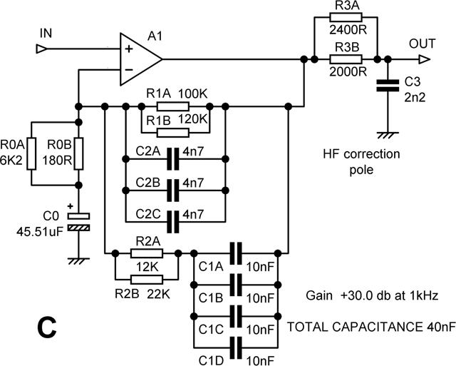
This process was applied to the C1= 3 x 10 nF amplifier in Figure 9.13, and the result is shown in Table 9.6 and Figure 9.15. The effective tolerances are shown in the rightmost column, and you can see that all of them are quite close to the best possible value of 0.577% (1/√3). This is a direct result of the extra freedom in design given by the use of the 3xE24 format.
RIAA Optimisation: C1 as 4 x 10 nF Capacitors, 3xE24
I also applied 3xE24 to the C1 = 4 x 10 nF design in Figure 9.14, and the result is shown in Figure 9.16. The table is omitted to save space.
In Electronics For Vinyl [1] a comprehensive table of component values and combinations are given for a gain at 1 kHz of +30 dB, +35 dB, and +40 dB. In each case, the same three options for C1 that we used for the +30 dB gain version here are offered, i.e. 3 x 10 nF, 1 x 33 nF, and 4 x 10 nF.
In the course of putting those tables, together 36 essentially random nominal resistor values were dealt with, and the average absolute error in nominal value if a single E96 resistor was used was 0.805%; for 2xE24 it was 0.285%, and for 3xE24 it was only 0.025%. So 2xE24 was three times better than 1xE96, and 3xE24 was 10 times better again. You have to use the absolute value of the error, as otherwise positive and negative errors tend to cancel out and give an unduly optimistic result. The RMS error could also be used, but it emphasises the larger errors, which may or may not be desirable.

Figure 9.16 Configuration C MM RIAA amplifier in Figure 9.14 (C1 = 4 x 10 nF) redesigned for 3xE24 parallel resistor combinations.
You may not agree that +30 dB (1 kHz) is the ideal gain for a phono amplifier. In Chapter 7 of Electronics For Vinyl [1], the component values are also given for +35 dB (1 kHz) and +40 dB (1 kHz). In each case, the same three options for C1 that we used for the +30 dB gain version are offered, i.e. 1 x 33 nF, 3 x 10 nF, and 4 x 10 nF. The nominal errors and effective tolerances are given for each component. Obviously this takes up a lot of room, and there is no space for it here.
Alternative optimisations of the RIAA networks shown here are possible. For example, we noticed that changing R0 from 200 Ω to 211.74 Ω had a negligible effect on the noise performance, worse by only 0.02 dB. That is well below the limits of measurement; what happens if we grit our teeth and accept a 0.1 dB noise deterioration? That is still at or below most measurement limits. It implies that R0 is 270 Ω, and the RIAA network impedance is therefore increased by 35%, so we could, for example, omit one of the 10 nF capacitors in Figure 9.14, naturally with suitable adjustments to other components, and so save some more of our hard-earned money.
To summarise, we have shown that there are very real differences in how efficiently the various RIAA networks use their capacitors, and it looks clear that using Configuration C rather than Configuration A will cut the cost of the expensive capacitors C1 and C2 in an MM stage by 36% and 19%, respectively, which I suggest is both a new result and well worth having. From there, we went on to find that different constraints on capacitor availability lead to different optimal solutions for Configuration C.
Both my Precision Preamplifier 96 [23] and the more recent Elektor Preamplifier 2012 [29] have MM stage gains close to +30 dB (1 kHz) like the examples given, but both use Configuration A, and five paralleled 10 nF capacitors are required.
I hope you will forgive me for not making public the software tools mentioned in this chapter. They are part of my stock in trade as a consultant engineer, and I have invested significant time in their development.
Switched-Gain MM RIAA Amplifiers
As noted, it is not necessary to have a wide range of variable or stepped gain if we are only dealing with MM inputs, due to the limited spread of MM cartridge sensitivities –only about 7 dB. According to Peter Baxandall, at least two gain options are desirable. [31]
However, as we have seen, the design of one-stage RIAA networks is not easy, and you might suspect that altering R0 away from the design point to change the gain is going to lead to some response errors. How right you are. Changing R0 introduces directly an LF RIAA error and indirectly causes a larger HF error, because the gain has changed, and so the HF correction pole is no longer correct. Here are some examples, where the RIAA components are calculated for a gain of +30 dB, with R0 = 200 Ω, and then the gain increased by a suitable reduction of R0:
- For +30 dB gain switched to +35 dB gain (R0 reduced to 112.47 Ω)
The RIAA LF error is +0.07 dB from 20 Hz–1 kHz
The HF error is -0.26 dB at 20 kHz.
- For +30 dB gain switched to +40 dB gain (R0 reduced to 63.245 Ω)
The RIAA LF error is +0.10 dB from 20 Hz–1 kHz
The HF error is -0.335 dB at 20 kHz.
These figures include the effect of finite open-loop gain when using a 5534A as the opamp; this increases the errors for the +40 dB gain option.
Thus for real accuracy, we need to switch not only R0 but also R1 in the RIAA feedback path and R3 in the HF correction pole; this would be very clumsy. If your RIAA error tolerance is a relaxed ±0.1 dB, switching R1 could be omitted, but two resistors still need to be switched. This assumes that the IEC Amendment is performed by a CR network after the MM stage, as described; this will be unaffected by changes in R0. Otherwise, if the IEC Amendment is implemented by a small value of C0, you would need to switch that component as well, to avoid gross RIAA errors below 100 Hz. All in all, switching the value of R0 is not an attractive proposition if you are looking for good accuracy.
There is a better way. If the gain is altered not by changing the value of R0 but instead keeping R0 constant and having a variable tap on it which feeds the inverting input of the amplifier, as in Figure 9.17, the loading of R0 on the rest of the RIAA network does not change with gain setting, and the RIAA response is accurate for all three settings.
You may be thinking ruefully that that is all very well, but we still need to switch the HF correction pole resistor so we get the proper correction for each gain. And yet, most elegantly, that is not the case. When we move the switch from +30 to +35, the value of the bottom feedback arm R0 is no longer R0A + R0B + R0C but is reduced to R0B + R0C, increasing the gain. R0A is now in the upper arm of the feedback network, and this causes the frequency response at HF to flatten out earlier than it would have done, in just the right way to keep the required HF correction pole unchanged. I won’t bore you with the mathematics, but you can prove it for yourself in 2 minutes with SPICE simulation. Likewise, switching to +40 dB leaves just R0C in the lower arm while R0A + R0B is in the upper arm. R4 maintains DC feedback when the switch is between contacts to prevent thunderous noises.

Figure 9.17 Configuration C MM amplifier with gain switchable to +30 dB, +35 dB, and +40 dB (1 kHz).
RIAA accuracy falls off slightly at LF for the +40 dB setting (– 0.3 dB at 20 Hz) because of the finite value of C0. Its value can be increased considerably if desired, as it has only the offset voltage across it, and a 6 V3 part will be fine.
Switched-Gain MM/MC RIAA Amplifiers
There is a considerable saving in parts if the same RIAA amplifier stage can be used for both MM and MC cartridges. This approach was used in many Japanese amplifiers, examples including the Pioneer A-8 (1981) and the Yamaha A-760, AX-500 (1987), AX-592, and AX-750. It implies that the gain of the stage must be increased by at least 20 dB in MC mode, which is more radical than the 5 dB or 10 dB gain changes examined in the previous section.
A typical arrangement is shown in Figure 9.18, which uses the same principle as Figure 9.17 with resistance removed from the bottom feedback arm being transferred to the top arm. The main difference is the very low value of R0B, which is essential, as its Johnson noise is effectively in series with the input, leading to a big C0 to maintain the LF response. R4 maintains DC feedback when the switch is between contacts to prevent horrible noises.

SPICE simulation shows that the RIAA accuracy is well within ±0.1 dB for the +30 dB setting. This is also true down to 40 Hz for the +50 dB setting, but the response then rolls off due to the finite value of C0, being 0.3 dB down at 20 Hz. C0 is already about as large as is practicable at 4700 μF/6 V3; at the time of writing, the smallest I found was 25 mm high and 10 mm diameter. Improving the +50 dB LF response, or switching to a higher gain, will require C0 to be replaced by a short circuit and DC conditions maintained by a servo. This approach is described in Chapter 11 on MC amplifiers in Electronics For Vinyl. [1]
If a BJT input device is used, there is the problem that the collector current needs to be low to get low current noise, which is essential for a good MM noise performance; on the other hand, the collector current needs to be high for low MC noise. The use of JFET input devices avoids this compromise, because the absence of current noise means a high drain current can be used in both cases; most of the amplifiers mentioned above used JFET input devices.
A significant complication is that the spread in sensitivity of MC cartridges is very much greater at about 36 dB than for MM cartridges (less than 10 dB), and having a single fixed MC gain is not very satisfactory.
Open-Loop Gain and RIAA Accuracy
There is no point in having a super-accurate RIAA network if the active element does not have enough open-loop gain to correctly render the response demanded. This was a major problem for two- and three-transistor discrete MM input stages, but one might have hoped that it would have disappeared with the advent of usable opamps. However, life is flawed, and gain problems did not wholly vanish. The TL072 was at one time widely used for MM inputs because of its affordability, even though its JFET input devices are a poor match to MM cartridge impedances, and its distortion performance was not the best. However, there was another lurking problem- not enough open-loop gain.
Even the open-loop gain of a 5534A is not adequate for a closed-loop gain of +40 dB at 1 kHz if you are aiming for an accurate RIAA response, and the +35 dB (1 kHz) situation is marginal. For +30 dB (1 kHz), the errors due to limited open-loop gain are negligible compared with the expected tolerances of the passive RIAA components. We have already seen that if a wide range of cartridges and recording levels are to be accommodated, the minimum gain should be no more than +30 dB (1 kHz), so this works out quite nicely.
Passive and Semi-Passive RIAA Equalisation
For many years, series-feedback RIAA preamplifiers as described earlier were virtually universal, it being accepted by all that they gave the best noise, overload performance, and economy, especially of active components. However, human nature being what it is, some people will always want to do things the hard way, and this is exemplified by the fashion for passive (actually, semi-passive is more accurate) RIAA equalisation. The basic notion is to split the RIAA equalisation into separate stages, and I have a dark and abiding suspicion that this approach may be popular simply because it makes the design of accurate RIAA equalisation much easier, as all you have to do is calculate simple time-constants instead of grappling with foot-long equations. There is a price, and a heavy one; the overload and/or noise performance is inevitably compromised.
Clearly a completely passive RIAA stage is a daft idea, because a lot of gain is required somewhere to get the 5 mV cartridge signal up to a usable amplitude. The nearest you can get to completely passive is the scheme shown in Figure 9.19a, where the amplification and the equalisation are wholly separate, with no frequency-dependent feedback used at all. R2, R3, and C1 implement T3 and T4, while C2 implements T5. There is no inconvenient T6 because the response carries on falling indefinitely with frequency. This network clearly gives its maximum gain at 20 Hz, and at 1 kHz it attenuates by about 20 dB. Therefore, if we want the modest +30 dB gain at 1 kHz used in the previous example, the A1 stage must have a gain of no less than 50 dB. A 5 mVrms 1 kHz input would therefore result in 1.58 V at the output of A1. This is only 16 dB below clipping, assuming we are using the usual sort of opamps, and an overload margin of 16 dB is much too small to be usable. It is obviously impossible to drive anything like a volume control or tone control stage from the passive network, so the buffer stage A2 is shown to emphasise that extra electronics are required with this approach.
The only way to improve the overload margin is to split the gain so that the A1 stage has perhaps 30 dB, while A2 after the passive RIAA network makes up the loss with 20 dB more gain. Sadly, this second stage of amplification must introduce extra noise, and there is always the point that you now have to put the signal through two amplifiers instead of one, so there is the potential for increased distortion.
The most popular architecture that separates the high and low RIAA sections is seen in Figure 9.19b. Here there is an active LF RIAA stage using feedback to implement T3 and T4 with R1, C1, R2, followed by R3, C2, which give a passive HF cut for T5. This is what I call an active-passive configuration. The values shown give an RIAA curve correct to within 0.04 dB from 20 Hz to 20 kHz. Note that because of the lack of time-constant interaction, we can choose standard values for both capacitors, but we are still left with awkward resistor values.
As always, amplification followed by attenuation means a headroom bottleneck, and this passive HF roll-off is no exception. Signals direct from disc have their highest amplitudes at high frequencies, so both these configurations give poor HF headroom, overload occurring at A1 output before passive HF cut can reduce the level. Figure 9.20 shows how the level at A1 output (Trace B) is higher at HF than the output signal (Trace A). The difference is Trace C, the headroom loss; from 1 dB at 1 kHz, this rises to 14 dB at 10 kHz and continues to increase in the ultrasonic region. The passive circuit was driven from an inverse RIAA network, so a totally accurate disc stage would give a straight line just below the +30 dB mark.
A related problem in this semi-passive configuration is that the opamp A1 must handle a signal with much more HF content than the opamp in the single-stage series-feedback configuration, worsening any difficulties with slew limiting and HF distortion. It uses two amplifier stages rather than one, and more precision components, because of the extra resistor. Another difficulty is that A1 is more likely to run out of open-loop gain or slew rate at HF, as the response plateaus above 1 kHz rather than being steadily reduced by increasing negative feedback. Once again, a buffer stage A2 is required to isolate the final time-constant from loading.
A third method of equalisation is shown in Figure 9.19c, where the T5 roll-off is done by feedback via R5, C2 rather than by passive attenuation. This is not really passive in any way, as the equalisation is done in two active stages, but it does share the feature of splitting up the time-constants for easier design. As with the previous circuit, A1 is running under unfavourable conditions, as it has to handle a larger HF content than in the series-feedback version, and there is now an inconvenient phase reversal. The values shown give the same gain and RIAA accuracy as the previous circuit, though in this case, the value of R3 can be scaled to change the gain.
There are many other alternative arrangements that can be used for passive or semi-passive equalisation. There could be a flat input stage followed by a passive HF cut and then another stage to give the LF boost, as in Figure 9.19d, which has even more headroom problems and uses yet more parts. I call this a passive-active configuration. In contrast, the “all-in-one-go” series feedback configuration avoids unnecessary headroom restrictions and has the minimum number of stages.
Passive RIAA is not an attractive option for general use, but it comes into its own in the archival transcription of recordings, where there are dozens of different pre-RIAA equalisation schemes, and it must be possible to adjust the turnover frequencies f3, f4, and f5 independently.
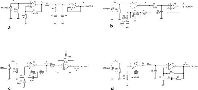
Peter Baxandall published a circuit in 1981 [31] with the configuration of Figure 9.19b that gave easy switched gain control and allowed the use of preferred values, with only two of them in the E24 series. Like all Peter’s ideas, it is well worth studying and is shown in Figure 9.21. The gains are +20, +30, and +40 dB, accurate to within ±0.3 dB; the switchable gain largely avoids the headroom problems of passive RIAA equalisation. The RIAA accuracy is within ±0.03 dB between 1 kHz and 20 kHz in each case, falling off to about -0,1 dB at 100 Hz. This is due to the way that R0 and C0 implement the IEC Amendment, giving f2 = 21.22 Hz rather than the correct 20.02 Hz; that is as close as you can get with a single 750 Ω E24 resistor for R0. It results in a response 0.34 dB too low at 20 Hz. The correct value for R0 is 795 Ω, so f2 could be made much more accurate by using the parallel pair 1 kΩ and 3.9 kΩ, which is only 0.1% too high. However, there is the tolerance of C0 to be considered, and when Peter was writing (1981), that would have been larger than we would expect today, so 750 Ω was probably considered to be close enough.
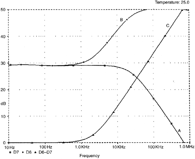
Figure 9.20 Headroom loss with passive RIAA equalisation. The signal level at A1 (Trace B) is greater than at A2 (Trace A), so clipping occurs there first. Trace C shows the headroom loss, which reaches 18 dB at 20 kHz.
As so often happens, what you think is a recent trend has its roots in the distant past. An active-passive MM input stage was published in Wireless World in 1961. [32] This had a two-transistor series-feedback amplifier which dealt with the LF equalisation, followed by a passive RC HF roll-off.
One problem with this circuit suggests itself. When the gain switch is between contacts, A1 has no feedback and will hit the rails. Very likely, Peter was thinking of a make-before break switch. The TDA1034B was an early version of the 5534 and capable of driving the relatively low impedance of the R2–C2 combination with low distortion.
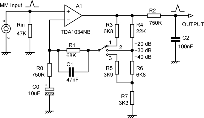
Figure 9.21 Active-passive RIAA stage with switched gain by Peter Baxandall.
MM Cartridge Loading and Frequency Response
The standard loading for a moving-magnet cartridge is 47 kΩ in parallel with a certain amount of capacitance, the latter usually being specified by the maker. The resulting resonance with the cartridge inductance is deliberately used by manufacturers to extend the frequency response, so it is wise to think hard before trying to modify it. Load capacitance is normally in the range 50 to 200 pF. The capacitance is often the subject of experimentation by enthusiasts, and so switchable capacitors are often provided at the input of high-end preamplifiers, which allow several values to be set up by combinations of switch positions. The exact effect of altering the capacitance depends on the inductance and resistance of the cartridge, but a typical result is shown in Figure 9.22, where increasing the load capacitance lowers the resonance peak frequency and makes it more prominent and less damped. It is important to remember that it is the total capacitance, including that of the connecting leads, which counts.
Because of the high inductance of an MM cartridge, adjusting the load resistance can also have significant effects on the frequency response, and some preamplifiers allow this too to be altered. The only objective way to assess the effects of these modifications is to measure the output when a special (and expensive) test disc is played.
When loading capacitance is used, it should be as near to the input socket as possible so it can contribute to filtering out RF before it radiates inside the enclosure. However, its effectiveness for EMC purposes is likely to be much compromised if the capacitors are switched. Normal practice is that the smallest capacitor is permanently in circuit, so it can be mounted right on the rear of the input socket. A continuously variable loading capacitance could be made with an old-style tuning capacitor (two-section for stereo); looking back, they were marvels of mass-produced precision engineering. The maximum value in an old medium-wave radio is often a rather convenient 500 pF. This would look well cool but naturally takes up a lot of space, and the variable-bootstrapping of a fixed capacitor (see the variable-frequency tone control in Chapter 15) would be much more compact.
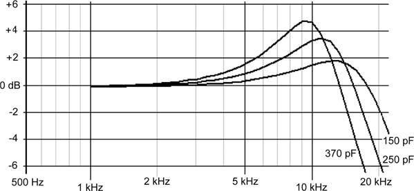
Figure 9.22 The typical effect of changing the loading capacitance on an MM cartridge.
The exact nature of this resonance does not have a consensus in the hi-fi community. There is also the possibility of what is usually called the “cantilever resonance”, which is a mechanical resonance between the effective tip mass of the stylus and the compliance of the vinyl it is tracking, the latter making up the spring part of the classic mass-and-spring system. The effective tip mass of the stylus is contributed to by the mass of the diamond tip, the cantilever, and the generator element on the other end, which may be a piece of iron, a magnet, or coils; it usually ranges from 0.2 to 0.7 milligrams. There is also the question of the contribution of the cantilever compliance and the possibility of a torsional resonance of the cantilever. [33] You are probably thinking by now that this is a mass of electromechanical compromises that should be left alone, and you are probably right.
MM Cartridge–Preamplifier Interaction
One often hears that there can be problems due to interaction between the impedance of the cartridge and the negative-feedback network. Most commentators are extremely vague as to what this actually means, but according to Tomlinson Holman [8], the factual basis is that it used to be all too easy to design an RIAA stage if you are using only two or three discrete transistors in which the NFB factor is falling significantly with frequency in the upper reaches of the audio band, perhaps due to dominant-pole compensation to achieve HF stability. (On the other hand, the amount of feedback is increasing with frequency due to RIAA equalisation.) Assuming a series-feedback configuration is being used, this means that the input impedance may fall with frequency, which is equivalent to having a capacitive input impedance. This interacts with the cartridge inductance and allegedly can cause a resonant peak in the frequency response, in the same way that cable capacitance or a deliberately added load capacitance can do.
For this reason, a flat-response buffer stage between the cartridge and the first stage performing RIAA equalisation was sometimes advocated. One design including this feature was the Cambridge Audio P50, which used a Darlington emitter-follower as a buffer; with this approach, there is an obvious danger of compromising the noise performance because there is no gain to lift the signal level above the noise floor of the next stage.
MM Cartridge DC and AC Coupling
Some uninformed commentators have said that there should be no DC blocking capacitor between the cartridge and the preamplifier. This is insane. Keep DC out of your cartridge. The signal currents are tiny (for MM cartridges 5 mV in 47 kΩ = 106 nA, while for MC ones 245 μV in 100 Ω = 2.45 μA, a good deal higher), and even a small DC bias current could interfere with linearity. I am not aware of any published work on how cartridge distortion is affected by DC bias currents, but I think it pretty clear they will not improve things and may make them very much worse. Large currents might partially demagnetise the magnet, be it moving or otherwise, ruining the cartridge. Even larger currents due to circuit faults might burn out the coils, ruining the cartridge even more effectively. You may call a lack of blocking capacitors high end, but I call it highly dangerous.
If I had a £15,000 cartridge (and they do exist, by Koetsu and Clearaudio), I would probably put two blocking capacitors in series. Or three. Well, actually, I’d probably sell it and buy a car.
Noise in MM RIAA Preamplifiers
Groove noise on a microgroove disc is between -70 and -64 dB (A-weighted) below the nominal level, as noted earlier. Later in this chapter, you will see that a humble 5534A in a single amplifier stage gives a signal/noise ratio of -81.4 dBA (A-weighted) without load-synthesis, which is only 3.1 dB worse than a wholly noiseless amplifier. The groove noise will therefore be 11.4 dB above the amplifier noise; even if we had magic noiseless electronics, the total noise level would only drop by 0.33 dB. This would be an argument against striving for low-noise amplifiers if it was an expensive pursuit, but it is not. All you need is a cheap opamp and a little ingenuity.
The basic noise situation for a series-feedback RIAA stage using an opamp is shown in Figure 9.23. The cartridge is modelled as a resistance Rgen in series with a significant inductance Lgen and is loaded by the standard 47 kΩ resistor Rin; this innocent-looking component causes more mischief than you might think. The amplifier A1 is treated as noiseless, its voltage noise being represented by the voltage generator Vnoise, and the current noise of each input being represented by the current generators Inoise+ and Inoise-, which are uncorrelated.
The contributions to the noise at the input of A1 are:
- The Johnson noise of the cartridge resistance Rgen. This sets the ultimate limit to the signal/noise ratio. The proportion of noise from Rgen that reaches the amplifier input falls with frequency as the impedance of Lgen increases. Here the fraction reaching the amplifier falls from 0.99 to 0.48 from 36 Hz to 17.4 kHz.
- The Johnson noise of the 47 kΩ input load Rin. Some of the Johnson noise generated by Rin is shunted away from the amplifier input by the cartridge, the amount decreasing with frequency due to the inductance Lgen. Here the fraction reaching the amplifier rises from 0.013 to 0.52 from 36 Hz to 17.4 kHz.
- The opamp voltage noise Vnoise. Its contribution is unaffected by other components.
- The noise voltage generated by Inoise+ flowing through the parallel combination of the cartridge impedance and Rin. This impedance increases with frequency due to Lgen. Here it increases from 619 Ω at 36 Hz to 24.5 kΩ at 17.4 kHz; the increase at the top end is moderated by the shunting effect of Rin. This increase has a major effect on the noise behaviour. For the lowest noise, you must design for a higher impedance than you might think, and Gevel [34] quotes 12 kΩ as a suitable value for noise optimisation.
- The Johnson noise of R0. For the values shown, and with A1 assumed to be 5534A, ignoring the Johnson noise of R0 improves the calculated noise performance by only 0.35 dB. The other resistors in the RIAA feedback network are ignored, as R0 has a much lower value.
- The noise voltage generated by Inoise- flowing through R0. For normal values of R0, say up to 1000 Ω, this contribution is negligible, affecting the total noise output by less than 0.01 dB.
Contributions 1, 2, and 4 are significantly affected by the rising impedance of the cartridge inductance Lgen with frequency. On top of this complicated frequency-dependent behaviour is overlaid the effect of the RIAA equalisation. This would reduce the level of white noise by 4.2 dB, but we are not dealing with white noise –the HF part of the spectrum has been accentuated by the effects of Lgen, and with the cartridge parameters given, RIAA equalisation actually reduces the noise amplitude by 10.4 dB.
The model as shown does not include the input DC blocking capacitor Cin. This needs to be 47 μF, or preferably 100uF, so that the voltage produced by the transistor noise current flowing through it is negligible.
Clearly this model has some quite complex behaviour. It could be analysed mathematically, using a package such as Math CAD, or it could be simulated by SPICE. The solution I chose is a spreadsheet mathematical model of the cartridge input, which I call MAGNOISE2.
Table 9.7 shows some interesting cases; output noise, EIN, and signal-to-noise ratio for a 5 mVrms input at 1 kHz are calculated for gain of +30.0 dB at 1 kHz. The IEC Amendment is included. The cartridge parameters were set to 610 Ω + 470 mH, the measured values for the Shure M75ED 2. Bandwidth is 22 Hz–22 kHz, no A-weighting is used, and 1/f noise is not considered. Be aware that the 5534A is a low-noise version of the 5534, with a typical voltage noise density of 3.5 rather than 4 nV√Hz and a typical current noise density of 0.4 rather than 0.6 pA/√Hz. The voltage noise and current noise densities used here are the manufacturer’s “typical” figures.
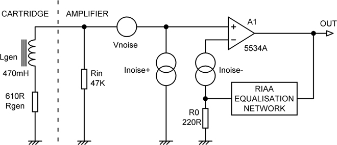
Figure 9.23 A moving-magnet input simplified for noise calculations, with typical cartridge parameter values (Shure ME75-ED2).
First, let us see how quiet the circuit of Figure 9.23 would be if we had miraculously noise-free electronics.
Case 0: We will begin with a completely theoretical situation with no amplifier noise and an MM cartridge with no resistance Rgen. Lgen is 470 mH. Rin is set to 1000 MΩ; the significance of that will be seen shortly. The noise out is a subterranean and completely unrealistic -136.8 dBu, and that is after +30 dB of amplification. This noise comes wholly from Rin and can be reduced without limit if Rin is increased without limit. Thus if Rin is set to 1000 GΩ, the noise out is -166.8 dBu.
You may ask why the noise is going up as the resistance goes down, whereas it is usually the other way around. This is because of the high cartridge inductance, which means the Johnson noise of Rin acts as a current rather than a voltage, and this goes up as the Rin resistance goes down.
Case 1: We now switch on the Johnson noise from Rgen (610 Ω). We will continue to completely ignore the cartridge loading requirements and leave Rin at 1000 MΩ, at which value it now has no effect on noise. The output noise with these particular cartridge parameters is then -98.8 dBu (Case 1a). This is the quietest possible condition (if you can come up with a noiseless amplifier), but you will note that right from the start, the signal/noise ratio of 85 dB compares badly with the 96 dB of a CD, a situation that merits some thought. And there is, of course, no groove noise on CDs. All of this noise comes from Rgen, the resistive component of the cartridge impedance. The only way to improve on this would be to select a cartridge with a lower Rgen but the same sensitivity or to start pumping liquid nitrogen down the tonearm. (As an aside, if you did cool your cartridge with liquid nitrogen at -196°C, the Johnson noise from Rgen would only be reduced by 5.8 dB, and if you are using a 5534A in the preamplifier, as in Case 10, the overall improvement would only be 0.75 dB. And, of course, the compliant materials would go solid and the cartridge wouldn’t work at all.)
With lower but still high values of Rin, the noise increases; with Rin set to 10 MΩ (Case 1b) the EIN is -128.7 dBu, a bare 0.1 dB worse. With Rin set to 1 MΩ (Case 1c), the EIN is now -128.2 dBu, 0.8 dB worse than the best possible condition (Case 1a).
| en | in | Rin | R0 | Noise output | S/N ref
5mV input |
EIN | NF ref Case 2 | Ref Case 10 | ||
|---|---|---|---|---|---|---|---|---|---|---|
| Case | Amplifier type | nV/rtHz | pA/rtHz | Ω | Ω | dBu | dB | dBu | dB | dB |
| 0 | Noiseless amp, no Rgen | 0 | 0 | 1000M | 0 | –136.8 | –123.1 | –166.8 | –41.2 | –44.3 |
| 1a | Noiseless amp | 0 | 0 | 1000M | 0 | –99.4 | –85.6 | –129.4 | –3.2 | –6.3 |
| 1b | Noiseless amp | 0 | 0 | 10M | 0 | –99.3 | –85.5 | –129.3 | ||
| 1c | Noiseless amp | 0 | 0 | 1M5 | 0 | –98.9 | –85.1 | –128.9 | ||
| 1d | Noiseless amp | 0 | 0 | 1M | 0 | –98.7 | –84.9 | –128.7 | ||
| 1e | Noiseless amp | 0 | 0 | 1M5 | 220 | –97.5 | –83.7 | –127.5 | ||
| 1f | Noiseless amp | 0 | 0 | 1M | 220 | –97.4 | –83.6 | –127.4 | ||
| 2 | Noiseless amp | 0 | 0 | 47k | 0 | –95.6 | –81.8 | –125.6 | 0 dB ref | –3.1 |
| 3 | Noiseless amp | 0 | 0 | 47k | 220 | –94.9 | –81.1 | –124.9 | 0.7 | –2.4 |
| 4a | 2SK710 FET, Id = 2 mA | 0.9 | 0 | 47k | 220 | –94.7 | –80.9 | –124.7 | 0.9 | –2.2 |
| 4b | J310 FET, Id = 10 mA | 2 | 0 | 47k | 220 | –94.2 | –80.4 | –124.2 | 1.4 | –1.7 |
| 5a | 2SB737 BJT, Ic=70uA | 1.75 | 0.39 | 47k | 220 | –93.6 | –79.8 | –123.6 | 2.0 | –1.1 |
| 5b | 2SB737 BJT, Ic=100uA | 1.47 | 0.46 | 47k | 220 | –93.4 | –79.6 | –123.4 | 2.2 | –0.9 |
| 6 | AD8656 * | 2.7 | 0 | 47k | 220 | –93.4 | –79.6 | –123.4 | 2.2 | –0.9 |
| 7 | 2SB737 BJT, Ic=200uA | 1.04 | 0.65 | 47k | 220 | –92.7 | –78.9 | –122.7 | 2.9 | –0.2 |
| 8 | OPA828 * | 4 | 0 | 47k | 220 | –92.7 | –78.9 | –122.7 | 2.9 | –0.2 |
| 9 | OPA2156 | 4 | 0.019 | 47k | 220 | –92.7 | –78.9 | –122.7 | 2.9 | –0.2 |
| 10 | 5534A BJT | 3.5 | 0.4 | 47k | 220 | –92.5 | –78.7 | –122.5 | 3.1 | 0 dB ref |
| 10a | 5534A BJT | 3.5 | 0.4 | 47k | 470 | –92.1 | –78.3 | –122.1 | 3.5 | +0.4 |
| 11 | OPA1642 JFET | 5.1 | 0.0008 | 47k | 220 | –91.8 | –78.0 | –121.8 | 3.8 | +0.7 |
| 12 | 5534A BJT | 3.5 | 0.4 | 47k | 1000 | –91.4 | –77.6 | –121.4 | 4.2 | +1.1 |
| 13 | OPA1622 | 2.8 | 0.8 | 47k | 220 | –91.4 | –77.6 | –121.4 | 4.2 | +1.1 |
| 14 | 5532A BJT | 5 | 0.7 | 47k | 220 | –90.5 | –76.5 | –120.5 | 5.1 | +2.0 |
| 15 | OPA2134 JFET | 8 | 0.003 | 47k | 220 | –89.3 | –75.5 | –119.3 | 6.3 | +3.2 |
| 16 | LM4562 BJT | 2.7 | 1.6 | 47k | 220 | –87.9 | –74.1 | –117.9 | 7.7 | +4.6 |
| 17 | LME49720 BJT | 2.7 | 1.6 | 47k | 220 | –87.9 | –74.1 | –117.9 | 7.7 | +4.6 |
| 18 | OPA604 JFET | 10 | 0.004 | 47k | 220 | –87.9 | –74.1 | –117.9 | 7.7 | +4.6 |
| 19 | OP275 BJT+JFET | 6 | 1.5 | 47k | 220 | –87.3 | –73.5 | –117.3 | 8.3 | +5.2 |
| 20 | AD797 BJT | 0.9 | 2 | 47k | 220 | –86.6 | –72.8 | –116.6 | 9.0 | +5.9 |
| 21 | TL072 JFET | 18 | 0.01 | 47k | 220 | –83.4 | –69.6 | –113.4 | 12.2 | +9.1 |
| 22 | LM741 BJT | 20 | 0.7 ** | 47k | 220 | –82.4 | –68.6 | –112.4 | 13.2 | +10.1 |
* No current-noise spec given by manufacturer’s data sheet. Presumed negligible.
** No current-noise spec. Derived from measurements.
Case 2: It is, however, a fact of life that MM cartridges need to be properly loaded, and when we set Rin to its correct value of 47 kΩ, things deteriorate sharply, the EIN rising by 3.2 dB (compared with Case 1a) to -125.6 dBu. That 47 kΩ resistor is not innocent at all. This case still assumes a noiseless amplifier and appears to be the appropriate noise reference for design, so the noise figure is 0 dB. (However, see the section on load synthesis later in this chapter, which shows how the effects of noise from Rin can be reduced by some non-obvious methods.) Cases 1a,b,c therefore have negative noise figures, but this has little meaning.
Case 3: We leave the amplifier noise switched off but add in the Johnson noise from R0 and the effect of Inoise- to see if the value of 220 Ω is appropriate. The noise only worsens by 0.7 dB, so it looks like R0 is not the first thing to worry about. Its contribution is included in all the cases that follow. The noise figure is now 0.7 dB.
We will now take a deep breath and switch on the amplifier noise.
Case 4: Here we use a single J310 FET, a device often recommended for this application. [34] With the drain current Id set to 10 mA, the voltage noise is about 2 nV√Hz; the current noise is negligible, which is why it is overall slightly quieter than the 2SB737 despite having more voltage noise.
Case 5: In these cases, a single discrete bipolar transistor is used as an input device, not a differential pair. This can give superior noise results to an opamp. The transistor may be part of a fully discrete RIAA stage or the front end to an opamp. If we turn a blind eye to supply difficulties and use the remarkable 2SB737 transistor (with Rb only 2 Ω typical), then some interesting results are possible. We can decide the collector current of the device, so we can to some extent trade off voltage noise against current noise, as described in Chapter 1. We know that current noise is important with an MM input, and so we will start off with quite a low Ic of 200 μA, which gives Case 7 in Table 9.7. The result is very slightly worse than the 5534A (Case 10). Undiscouraged, we drop Ic to 100 μA (Case 5b), and voltage noise increases but current noise decreases, the net result being that things are now 0.9 dB quieter than the 5534A. If we reduce Ic again to 70 μA (Case 5a), we gain another 0.2 dB, and we have an EIN of -123.6 and a noise figure of only 2.0 dB. Voltage noise is now increasing fast, and there is virtually nothing to be gained by reducing the collector current further. The 2SB737 is now obsolete. For information on replacements, see Chapter 10.
We therefore must conclude that even an exceptionally good single discrete BJT with appropriate support circuitry will only gain us a 1.1 dB noise advantage over the 5534A, while the J310 FET gives only a 1.7 dB advantage, and it is questionable if the extra complication is worth it. You are probably wondering why going from a single transistor to an opamp does not introduce a 3 dB noise penalty because the opamp has a differential input with two transistors. The answer is that the second opamp transistor is connected to the NFB network and sees much more favourable noise conditions, a low and resistive source impedance in the shape of R0.
Case 6: The AD8656 is a relatively new opamp (released 2005) and gives the best noise results so far for an IC due to its low voltage noise of 2.7 nV/√Hz. However, it is only 0.9 dB quieter than the venerable (and cheap) 5534A. It makes you think…
Case 7: This is the 2SB737 with an Ic of 200 μA; see Case 5.
Case 8: The OPA828 is a new JFET-input opamp (released 2018).
Case 9: The OPA2156 is a new CMOS opamp (released 2018).
Case 10: Here we have a 5534A as the amplifying element, and using the typical 1 kHz specs for the A-suffix part, we get an EIN of -122.5 dBu and an NF of 3.1 dB. R0 is 220 Ω. Using thoroughly standard technology and one of the cheapest opamps about, we are within three decibels of perfection; the only downside is that the opportunities for showing off some virtuoso circuit design with discrete transistors appear limited. Case 10 is useful as a standard for comparison with other cases, as in the rightmost column of Table 9.7.
How does the value of R0 affect noise? In Case 10a, R0 is increased to 470 Ω, and the noise is only 0.4 dB worse; if you can live with that, the increase in the impedance of the RIAA feedback network allows significant savings in expensive precision capacitors. Reducing R0 from 220 Ω to 100 Ω is do-able at some cost in capacitors but only reduces the noise output by 0.2 dBu. The value of R0 can be manipulated to get convenient capacitor values in the RIAA network, because it has only a weak effect on the noise performance (see section on RIAA equalisation).
We have seen that the presence of Lgen has a big effect on the noise contributions. If we reduce Lgen to zero, the noise out drops from -92.5 to -94.7 dBu. Halving it gives -93.8 dBu. Minimum cartridge inductance is good.
What about Rgen? With the original value of Lgen, setting Rgen to zero only reduces the noise from -92.5 to -93.5 dBu; the cartridge inductance has more effect than its resistance.
Case 11: The OPA1642 is a JFET-input opamp with noise densities of 5.1 nV/√Hz for voltage and a startlingly low 0.0008 pA/√Hz for current. This modern JFET technology gives another way to get low MM noise –accept a higher en in order to get a very low in. The OPA1642 gives an EIN of -121.8 dBu, beating the 5532 but not the 5534A with R0 = 220 Ω. At the time of writing, the OPA1642 is something like 20 times more expensive than the 5532.
Case 12: We go back to the 5534A with R0 now raised substantially further to 1000 Ω, and the noise is only 1.1 dB worse than the 5534A 220 Ω case. This shows that the value of R0 is not critical.
Case 13: The OPA1622 is a relatively new (released 2016) BJT-input opamp. Its current-noise is twice that of the 5534A, and its place in the table suffers accordingly.
Case 14: It is well known that the single 5534A has somewhat better noise specs than the dual 5532A, with both en and in being significantly lower, but does this translate into a significant noise advantage in the RIAA application? Case 14 shows that on plugging in a 5532A, the noise output increases by 2.0 dB, the EIN increasing to -120.5 dBu. The NF is now 5.1 dB, which looks a bit less satisfactory. If you want good performance, then the inconvenience of a single package and an external compensation capacitor are well worth putting up with.
Case 15: Here we try out the FET-input OPA2134; the en is much higher at 8 nV√Hz, but in is very low indeed at 3 fA√Hz. The greater voltage noise does more harm than the lower current noise does good, and the EIN goes up to -119.3 dBu. The OPA2134 is therefore 3.2 dB noisier than the 5534A and 2.5 dB noisier than the 5532A; and it is not cheap. The noise figure is now 6.3 dB, which to a practised eye would show that something had gone amiss in the design process.
Case 16: The LM4562 BJT-input opamp gives significant noise improvements over the 5534/5532 when used in low-impedance circuitry, because its en is lower at 2.7 nV√Hz. However, the impedances we are dealing with here are not low, and the in, at 1.6 pA√Hz, is 4 times that of the 5534A, leading us to think it will not do well here. We are sadly correct, with EIN deteriorating to -117.9 dBu and the noise figure an unimpressive 7.7 dB. The LM4562 is almost 5 dB noisier than the 5534A and, at the time of writing, is a lot more expensive. Measurements confirm a 5 dB disadvantage.
Case 17: The LME49720 is a recent (released 2007) BJT-input opamp with the same voltage and current densities as the LM4562 and so gives the same EIN of -117.9 dBu, 5 dB noisier than the 5534A.
Case 18: The OPA604 is a FET-input opamp that is often recommended for MM applications by those who have not studied the subject very deeply. It has a high voltage noise density of 10 nV/√Hz for voltage and a low 0.004 pA/√Hz for current-noise. This different balance of voltage and current noise gives the same EIN of 117.9 dBu as Case 17, 5 dB noisier than the 5534A.
Case 19: The OP275 has both BJT and FET input devices. Regrettably, this appears to give both high voltage noise and high current noise, resulting in a discouraging EIN of -117.3 dBu, and a noise figure of 8.2 dB. It is 5.2 dB noisier than a 5534A in the same circuit conditions. Ad material claims “excellent sonic characteristics”, perhaps in an attempt to divert attention from the noise. It is expensive.
Case 20: The AD797 has very low voltage noise because of its large BJT input transistors, but current noise is correspondingly high, and it is noisy when used with an MM cartridge. And it is expensive, especially so since it is a single opamp with no dual version. Definitely not recommended for MM; allegedly useful in submarines (for sonar).
Case 21: The TL072 with its FET input has very high voltage noise at 18 nV√Hz but low current noise. We can expect a poor performance. We duly get it, with EIN rising to -113.4 dBu and a very indifferent noise figure of 12.2 dB. The TL072 is 9.1 dB noisier than a 5534A and 8.4 dB noisier than a 5532A. The latter figure is confirmed (within experimental error, anyway) by the data listed in the section that follow son noise measurements. There is no reason to use a TL072 in an MM preamp; it must be one of the worst you could pick.
Case 22: Just for historical interest, I tried out the LM741. Voltage noise measures about 20 nV√Hz. I have no figures for the current noise, but I think it’s safe to assume it won’t be better than a 5532, so I have used 0.7 pA√Hz. Predictably, the noise is the highest yet, with an EIN of -112.4 dBu, but it is a matter for some thought that despite using a really ancient part, it is only 10 dB worse than the 5534A. The noise figure is 13 dB.
Hybrid MM Amplifiers
In Table 9.7, the noise results are shown for single discrete devices as well as opamps. These cannot be used alone in a phono amplifier because of the need for both substantial open-loop gain and good load-driving ability. The discrete device can be used as the first stage of a discrete amplifier, as described in Chapter 10, but it is more convenient to combine the discrete device with an opamp, which will give both the open-loop gain and the load-driving ability required at lower cost and using less PCB area. Either a BJT or a JFET may be used as the device, given suitable biasing. The 5532 or 5534 is once again a suitable opamp.
Figure 9.24 shows a basic arrangement. For optimal noise, the Ic of Q1 will probably be in the range 50–200 μA, and most of this is supplied through R8. While there is always a DC path through the RIAA network because of the need to define the LF gain, trying to put all of the Ic through it would lead to an excessive voltage drop, which would appear as a big offset at the output. Instead, the DC flowing through R1 is just used for fine-tuning of Q1 operating conditions by negative feedback. This means that if R8 and Vbias are correctly chosen, there might be a few 100mV of offset either way at the opamp output. This is not large enough to significantly affect the output swing, but it needs blocking; C5 is shown as non-polar to emphasise the point that the offset might go either way.
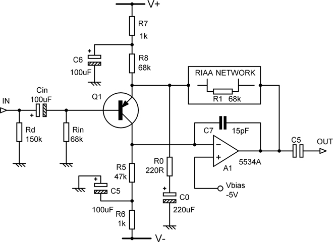
Figure 9.24 Basic arrangement of a hybrid MM phono amplifier with typical values. Note non-polar output blocking cap.
C7 gives dominant-pole compensation of the loop; the RIAA usually causes the closed-loop gain to fall to unity at high frequencies (but see the section on switched-gain phono amps in Chapter 7), and achieving HF stability may require some experimentation with its value. The two supply rails are heavily filtered by R6, C5 and R7, C6 to keep out ripple and noise; no fancy low-noise supply is needed; 78/79 series regulators work just fine.
Balanced MM Inputs
So far, all the MM amplifiers considered have been of the usual unbalanced input type. There is a reason for this.
There is some enthusiasm out there for balanced MM inputs, on a “me-too!” basis, because balanced inputs are almost universally used in professional audio, for excellent reasons. However, an MM cartridge and its short connecting lead (short to control shunt capacitance) are nothing like the average professional connection that links two pieces of powered equipment and so is likely to have nasty currents flowing through its ground wire. The coils of an MM cartridge are floating, or should be; connecting one side to the turntable ground is likely to cause hum. How might common-mode interference, which is what balanced inputs reject, get into the cartridge or lead?
- Electrical fields into the cartridge. Any sensible cartridge is electrically shielded, so balancing is not required. For electrically unscreened cartridges (there is one brand that is globally famous for humming), the coupling will not be identical for the two ends of the coil, so it won’t be a true common mode signal; I dare say you could have a “balanced” input in which you set the gain of hot and cold inputs separately so you could try to null the hum. Good luck getting that to stay nulled as the arm moves across the disk; this is not an idea to pursue.
- Magnetic fields into the cartridge. These will cause a differential voltage across the floating cart coil, just as for the signal, and will not be rejected in any way by a balanced input.
- Electrical or magnetic coupling into the cable. Negligible with usual cable lengths and even half-sensible cable layout; i.e. keep it away from mains wiring and transformers. A balanced input is therefore not required.
These points were debated at length on DIYaudio, and no evidence was offered that they were wrong. For this reason, balanced MM inputs receive only limited attention here.
Noise in Balanced MM Inputs
When dealing with line inputs, a balanced input is much noisier than an unbalanced input (see Chapter 18). The conditions for an MM balanced input are quite different, but it still seems highly likely that it will be noisier because two (or more) amplifiers are used rather than one, and we don’t want a noise penalty if there are no countervailing benefits. Let’s find out…
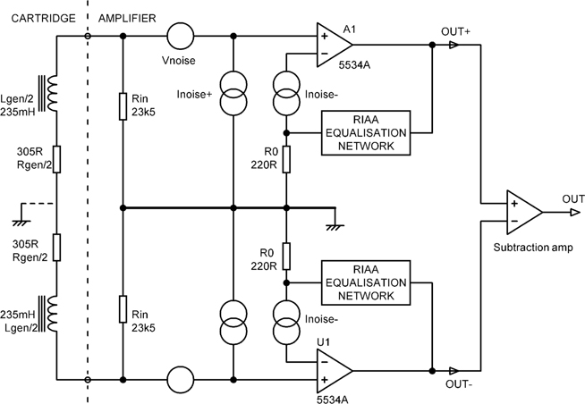
Figure 9.25 A balanced MM input using two 5534A stages with their outputs subtracted.
Figure 9.25 depicts a balanced MM input made up of two 5534A stages with their outputs subtracted (or “phase summed”). All the noise sources are shown. The equal loading on each cartridge pin makes the coil appear balanced to the amplifiers; the “ground” at the midpoint of the cartridge is purely notional, with no physical connection there.
Therefore, the 47 kΩ load is split into two 23.5 kΩ resistances; these give less Johnson noise by a factor of √2, and also the voltage produced by Inoise+ will be halved. The Vnoise is unaffected, and we now have two uncorrelated sources of it.
The unweighted noise output for a standard unbalanced 5534A amplifier in a +30 dB (1 kHz) amplifier is -92.51 dBu, as in Table 9.7. Cartridge parameters are 610 Ω + 470 mH. Reducing Rin to 23.5 kΩ and changing the cartridge parameters to 305 Ω + 235 mH, as we are only dealing with half of the cartridge, reduces the noise output to -94.36 dBu. We then have to subtract the outputs of the two sides, which is equivalent to summing their noise. Neglecting the noise of the subtracting amplifier, which is quite realistic given the relatively high noise output of the input stages, the result is -91.36 dBu. This is only 1.1 dB noisier than an unbalanced input and would be quite acceptable if a balanced input solved other problems, but as noted, I’ve yet to hear any convincing argument that it does.
The arrangement of Figure 9.25 is an illustration of principle and is not claimed to be optimal. For one thing, there are two RIAA networks, and they are very likely the most expensive part of the circuit. They will have to be accurate for accurate RIAA, and that may well be enough to give a good practical CMRR if you can find a use for it. The arrangement uses two opamps, effectively putting four input devices in series in the input circuit, though the two on the opamp inverting inputs see benign noise conditions because of the low resistance of R0. This could be addressed by using an instrumentation amplifier IC, but the possible noise advantage is small.
Noise Weighting
The frequency response of human hearing is not flat, especially at lower listening levels. Some commentators therefore feel it is appropriate to use psychoacoustic weighting when studying noise levels. This is almost invariably ANSI A-weighting despite the fact that it is generally considered inaccurate, undervaluing low frequencies. ANSI B-, C-, and D-weightings are not used in audio. The ITU-R ARM 468 weighting (CCIR-468) is a later development and generally considered to be much better but is only rarely used in audio (ARM stands for average-responding meter). I prefer unweighted measurements, as you are one step closer to the original data. Full details of both methods, with circuitry to implement them, are given in Electronics For Vinyl. [1]
Noise Measurements
In the past, many people who should have known better have recommended that MM input noise should be measured with a 1 kΩ load, presumably thinking that this emulates the resistance Rgen, which is the only parameter in the cartridge actually generating noise –the inductance is, of course, noiseless. This overlooks the massive effect that the inductance has in making the impedance seen at the preamp input rise with frequency, so that at higher frequencies, most of the input noise actually comes from the 47 kΩ loading resistance. I am grateful to Marcel van de Gevel for drawing my attention to some of the deeper implications of this point. [34]
The importance of using a real cartridge load is demonstrated in Table 9.8, where the noise performance of a TL072 and a 5532 are compared. The TL072 result is 0.8 dB too low and 5532 result 4.9 dB too low –a hefty error. In general, results with the 1 kΩ resistor will always be too low, by a variable amount. In this case you still get the right overall answer – i.e. you should use a 5532 for least noise –but the dB difference between the two has been exaggerated by almost a factor of two, by undervaluing the 5532 current noise.
Amplifier gain was +29.55 dB at 1 kHz. Bandwidth was 400–22 kHz to remove hum, rms sensing, no weighting, cartridge parameters 610 Ω + 470 mH.
| Zsource | TL072 | 5532 | 5532 benefit | 5532 EIN |
|---|---|---|---|---|
| 1 kΩ resistor | –88.0 | –97.2 dBu | +9.8 dB | –126.7 dBu |
| Shure M75ED 2 | –87.2 | –92.3 dBu | +5.1 dB | –121.8 dBu |
Cartridge Load Synthesis for Lower Noise
Going back to Table 9.7, you will recall that when we were examining the situation with the amplifier and feedback network noise switched off, adding in the Johnson noise from the 47 kΩ loading resistor Rin caused the output noise to rise by 3.2 dB. In real conditions with amplifier noise included, the effect is obviously less dramatic, but it is still significant. For the 5534A (Case 10), the removal of the noise from Rin (but not the loading effect of Rin) reduces the noise output by 1.3 dB. Table 9.9 summarises the results for various amplifier options; the amplifier noise is unaffected, so the noisier the technology used, the less the improvement.
This may appear to be utterly academic, because the cartridge must be loaded with 47 kΩ to get the correct response. This is true, but it does not have to be loaded with a physical 47 kΩ resistor. An electronic circuit that has the V/I characteristics of a 47 kΩ resistor, but lower noise, will do the job very well. Such a circuit may seem like a tall order –it will after all be connected at the very input, where noise is critical –but unusually, the task is not as difficult as it seems.
| Rin =47KΩ | Rin =1M | Synth
advantage |
Rin =1M5 | Synth advantage | |||||
|---|---|---|---|---|---|---|---|---|---|
| Case | Amplifier type | EIN dBu | NF dB | EIN dBu | NF dB | dB | EIN dBu | NF dB | dB |
| 4a | 2SK710 FET, Id = 2 mA | –124.7 | 3.5 | –127.1 | 1.1 | 2.9 | –127.3 | 1.3 | 3.1 |
| 4b | J310 FET, Id = 10 mA | –124.2 | 4.0 | –126.3 | 1.9 | 2.5 | –126.4 | 2.0 | 2.6 |
| 5a | 2SB737 70uA | –123.6 | 4.6 | –125.3 | 2.9 | 1.7 | –125.4 | 3.0 | 1.8 |
| 5b | 2SB737 100uA | –123.4 | 4.8 | –125.1 | 3.1 | 1.7 | –125.2 | 3.2 | 1.8 |
| 7 | 2SB737 200uA | –122.7 | 5.5 | –124.1 | 4.1 | 1.4 | –124.2 | 1.5 | 1.5 |
| 10 | 5534A | –122.5 | 5.7 | –123.8 | 4.4 | 1.3 | –123.9 | 1.4 | 1.4 |
| 14 | 5532A | –120.5 | 7.7 | –121.3 | 6.9 | 0.8 | –121.4 | 7.0 | 0.9 |
| 15 | OPA2134 | –119.3 | 8.9 | –119.9 | 8.3 | 0.6 | –119.9 | 8.3 | 0.6 |
| 16 | LM4562 | –117.9 | 10.3 | –118.3 | 9.9 | 0.4 | –118.4 | 10.0 | 0.5 |
| 21 | TL072 | –113.4 | 14.8 | –113.5 | 14.7 | 0.1 | –113.5 | 14.7 | 0.1 |
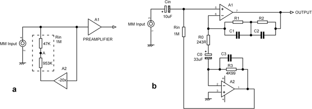
Figure 9.26 Electronic load synthesis: a) the basic principle; b) the Gevel circuit.
Figure 9.26a shows the basic principle. The 47 kΩ Rin is replaced with a 1 MΩ resistor whose bottom end is driven with a voltage that is phase inverted and 20.27 times that at the top end. If we conceptually split the 1 MΩ resistor into two parts of 47 kΩ and 953 kΩ, a little light mathematics shows that with -20.27 times Vin at the output of A2, the voltage at the 47 kΩ–953 kΩ junction A is zero, and so as far as the cartridge is concerned, it is looking at a 47 kΩ resistance to ground. However, the physical component is 1 MΩ, and the Johnson current noise it produces is less than that from a 47 kΩ (Johnson current noise is just the usual Johnson voltage noise applied through the resistance in question). The point here is that the apparent resistor value has increased by 21.27 times, but the Johnson noise has only increased by 4.61 times because of the square root in the Johnson equation; thus the current noise injected by Rin is also reduced by 4.61 times. The noise reduction gained with a 5534A (Case 10) is 1.3 dB, which is very close to the 1.5 dB improvement obtained by switching off the Rin noise completely. If a resistor larger than 1 MΩ is used, slightly more noise reduction can be obtained, but that would need more gain in A2, and we would soon reach the point where it would clip before A1, restricting headroom. In this case, with a gain of 21 times, we get a very good noise figure of 1.8 dB, though the lowest noise output comes from the 2SB737 at 70 μA.
The implementation made known by Gevel [11] is shown in Figure 9.26b. This ingenious circuit uses the current flowing through the feedback resistor R0 to drive the A2 shunt feedback stage. With suitable scaling of R3 (note that here it has an E96 value), the output voltage of A2 is at the right level and correctly phase inverted. When I first saw this circuit, I had reservations about connecting R0 to a virtual ground rather than a real one and thought that extra noise from A2 might find its way back up R0 into the main path. (I hasten to add that these fears may be quite unjustified, and I have not found time so far to put them to a practical test.) The inverting signal given by this circuit is amplified by 20.5 times rather than 20.27, but this has a negligible effect on the amount of noise reduction.
Because of these reservations, I tried out my version of load synthesis as shown in Figure 9.27. This uses the basic circuit of Figure 9.26a; it is important that the inverting stage A3 does not load the input with its 1 kΩ input resistor R4, so a unity-gain buffer A2 is added. The inverting signal is amplified by 20 times, not 20.27, but once again this has negligible effect on the noise reduction.
In practical measurements with a 5534A as amplifier A1, I found that the noise improvement with a real cartridge load (Shure M75ED 2, cartridge parameters 610 Ω + 470 mH) was indeed 1.3 dB, just as predicted, which is as nice a matching of theory and reality as you are likely to encounter in this world. There were no HF stability problems. Whether the 1.3 dB is worth the extra electronics is a good question; I say it’s worth having.
When measuring the effect of load synthesis, it is highly convenient to be able to switch immediately between normal and synthesised modes. This can be done with one link, as in Figure 9.27. Adding link J1 loads the input with the physical 47 kΩ resistor Rin1 and at the same time short-circuits the output of A3 to ground. The 953 kΩ resistor Rin2 is made up of two E24 resistors in parallel, giving a combined value only 0.26% below nominal.
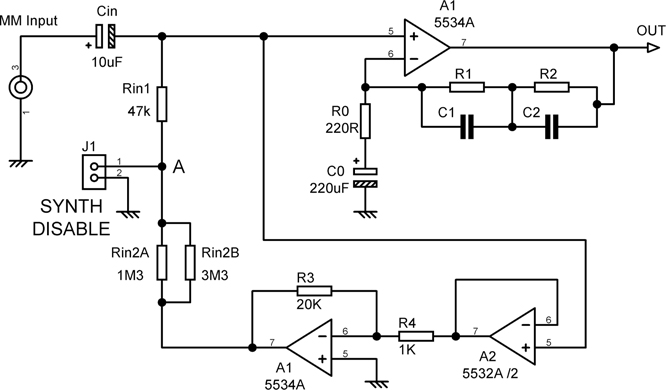
Subsonic Filters
In the earliest parts of this chapter, we have seen that the worst subsonic disturbances occur in the 2–4 Hz region due to disk warps and are about 8 dB less at 10 Hz. We have also seen that the IEC Amendment gives only 14 dB of attenuation at 4 Hz and, in any case, is often omitted by the manufacturer or switched out by the user. It is therefore important to provide authoritative subsonic filtering. We want frequencies around 10 Hz to be attenuated by at least 40 dB. What needs to be settled is what order and what kind of filter to use, because some people at least will be concerned about the audibility of LF phase shifts and how far into the audio band the filter should intrude. There is nothing approaching a consensus on either point, so it can be a wise move to configure the subsonic filter so it can be switched out.
Subsonic Filtering: Butterworth Filters
High-pass filters used for RIAA subsonic are typically of the second-order or third-order Butterworth (maximally flat) configuration, rolling off at rates of 12 dB/octave and 18 dB/octave, respectively. Fourth-order 24 dB/octave filters are much less common, presumably due to needless worries about the possible audibility of rapid phase changes at the very bottom of the audio spectrum. The responses of Butterworth filters from the second to the sixth order are shown in Figure 9.28. They are called all-pole filters, which is rather technical but means that the response is monotonic, always going downward once it has started to do so.
The well-known Sallen and Key configuration is very handy for this sort of filter. A second-order Sallen and Key is simple to design; the two series capacitors C1 and C2 are made equal, and R2 is made twice the value of R1. Such a filter with a -3 dB point at 20 Hz is shown in Figure 9.29a. Other roll-off frequencies can be obtained simply by scaling the component values while keeping C1 equal to C2 and R2 twice R1. The response is 24.0 dB down at 5 Hz, by which time the 12 dB/octave slope is welle stablished, and we are well protected against disk warps. It is, however, only 12.3 dB down at 10 Hz, which gives little protection against arm-resonance problems. Above the -3 dB roll-off point, the response is still -0.78 dB down at 30 Hz, which is intruding a bit into the sort of frequencies we want to keep. We have to conclude that a second-order filter really does not bifurcate the condiment, and the faster roll-off of a third-order filter is preferable.
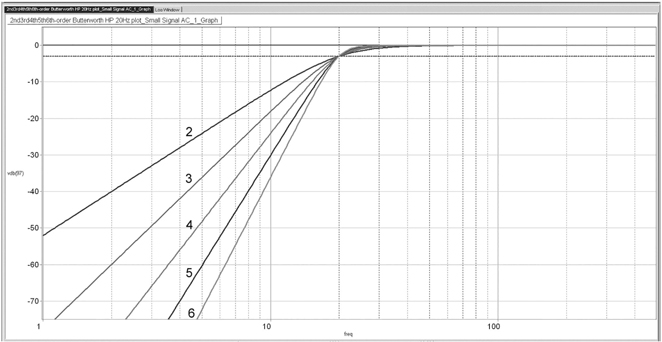
Third-order filters are a little more complex. In general, they consist of a second-order filter cascaded with a first-order roll-off, using two opamp sections. It can, however, be done with just one, as in Figure 9.29b, which is a third-order Butterworth filter also with a -3 dB point at 20 Hz. The resistor value ratios are now a less friendly 2.53:1.00:17.55, and the circuit shown uses the nearest E24 values to this –which, by happy chance, come out as E12 values. The frequency response is shown in Figure 9.28, where it can be seen to be 18.6 dB down at 10 Hz, which should keep out any arm-resonance frequencies. It is 36.0 dB down at 5 Hz, so disk warp spurii won’t have a chance. The 30 Hz response is now only down by an insignificant -0.37 dB, which demonstrates how a third-order filter is much better than a second-order filter for this application. As before, other roll-off frequencies can be had by scaling the component values while keeping the resistor ratios the same.
Because of the large capacitances, the noise generated by the resistors in a high-pass filter of this sort is usually well below the opamp noise. The capacitances do not, of course, generate any noise themselves. With the values used here, SPICE simulation shows that the resistors produce -125.0 dBu of noise at the output (22 kHz bandwidth, 25°C). The use of the LM4562 will reduce voltage-follower CM distortion compared with the 5534/5532 but may be noisier in some cases due to the higher current noise of the LM4562.
Capacitor distortion in electrolytics is (or should be) by now a well-known phenomenon. It is perhaps less well known that non-electrolytics can also generate distortion in filters like these. This has nothing to do with subjectivist musicality, but it is all too real and measurable. Details of the problem are given in Chapter 2, where it is concluded that only NP0 ceramic, polystyrene, and polypropylene capacitors can be regarded as free of this effect. The capacitor sizes needed for subsonic filters are large if impedances and hence noise are to be kept low, which means it has to be polypropylene. As a result, anything larger than 470 nF gets to be big and expensive, so that is the value used here. 220 nF polypropylene is substantially smaller and about half the price; use it if you can. There is more information on this, and on high-pass filters in general, in Chapter 6 on filters.
At the start of this section, we decided that a really good subsonic filter should be down -40 dB around 10 Hz, but we’re clearly not going to get it with either of the two all-pole filters examined so far. They are useful filters and very much better than nothing, but they do not meet this rather severe criterion. A seventh-order Butterworth should do it, with a small safety margin of 2 dB, but that means a four-stage filter, which is a relatively complex design and may have problems with component sensitivities. Increasing the safety margin beyond 2 dB means an 8th-order Butterworth, and that is getting into difficult territory.
Subsonic Filtering: Elliptical Filters
As we’ve seen earlier in this chapter, ideally we would like the cart/arm resonance frequencies in the band 8–12 Hz to be attenuated by -40 dB, with 2–4 Hz also getting good suppression. All-pole filters can’t do that without unduly encroaching on the passband and/or being unduly complex. An alternative approach is to use a notch filter that, in theory at least, gives infinite attenuation in the centre of the notch. To make a notch filter, zeros are added to the filter poles; there isn’t space to explain that further, but see any filter textbook.
Chebychev filters have faster roll-off than Butterworth but introduce ripples into the passband response, which are really unhelpful if you are looking for accurate RIAA equalisation. More useful is the Inverse Chebychev, which also has a faster roll-off than Butterworth but still has a maximally flat passband with no ripples. There are one or more notches in the stopband, and one of them can be plonked exactly on 10 Hz. The price of this useful behaviour is that the stopband gain keeps bouncing back up again between the notches, but it will not exceed a level A0 chosen at the design stage; here it is -35 dB. However, when it comes to design information, the Inverse Chebychev high-pass is the redheaded stepchild of filters, and so I had to design it as a more general elliptical filter with passband ripple set to zero, and this is (I think) exactly the same as an Inverse Chebychev. The word “elliptical” comes from the underlying mathematics, which is fearsome and has only the remotest connection with geometrical ellipses. Elliptical-shaped PCBs are not required.
There is little point in trying to guess exactly which cart/arm combination on the market gives the worst subsonics, so I put the notch at 10 Hz, with due attention paid to how much it attenuates from 8–12 Hz. A very narrow notch would not be useful, as it cannot deal with cart/arm variations. You can always make a notch rumble filter by taking a third-order Butterworth and cascading it with a standard symmetrical 10 Hz notch filter, but it is not efficient and no way to design filters. A true filter cunningly fits together the various peakings and roll-offs of its cascaded stages to make the overall turnover and roll-off as clean and steep as possible.
EFV [1] contains much more explanation and detail; suffice it to say that after a lot of study, I decided that a fourth-order classical (non-MCP) filter was a good compromise between parts cost and effectiveness. Even-order filters of this type are better because they have an ultimate roll-off of 12 dB/octave, giving better suppression of very low frequencies around 2–4 Hz, while odd-order filters only give an ultimate roll-off of 6 dB/octave.
Figure 9.30 shows the response of the fourth-order classical high-pass elliptical filter with A0= -35 dB. The -3 dB frequency is 21.0 Hz, very close to that of the third-order Butterworth. The -0.1 dB frequency is 30.5 Hz, so there is minimum intrusion into the passband. The notch bandwidth at -35 dB is 8.5–10.9 Hz. The attenuations at some important frequencies are given in Table 9.10.
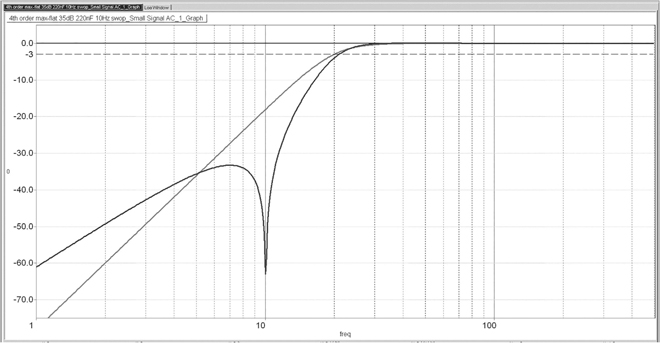
| Freq | 1 Hz | 5 Hz | 10 Hz | 20 Hz | 30 Hz | -3 dB freq | -0.1 dB freq |
|---|---|---|---|---|---|---|---|
| Elliptical fourth–order classic | –61 dB | –35.7 dB | –70 dB | –4.0 dB | –0.14 dB | 21.0 Hz | 30.5 Hz |
| Third–order Butterworth | –78 dB | –36 dB | –18 dB | –3.0 dB | –0.37 dB | 20 Hz | 37 Hz |
| Fourth–order Butterworth | –104 dB | –48 dB | –24 dB | –3.0 dB | –0.16 dB | 20 Hz | 32 Hz |
The response around 8–12 Hz is far superior for the elliptical filter, though its attenuation in the 2–4 Hz region is between 3 and 10 dB worse. If -50 dB at 2 Hz is not enough, an extra second-order high-pass filter with a cutoff around 4 Hz would make the elliptical filter as good as the third-order Butterworth in the 1–4 Hz region. Alternatively, you could do something about that record deck.
The fourth-order elliptical filter consists of a second-order high-pass filter A4 followed by a Bainter high-pass-notch filter A1–A3. Putting the high-pass stage first makes internal clipping in the Bainter filter less likely. Figure 9.31 uses 2xE24 resistor combinations and 220 nF capacitors. Polypropylene capacitors must be used to get the lowest distortion.
EFV contains a long chapter on subsonic filtering, including many kinds of Butterworth and elliptical filters up to sixth order. I think I can say without fear of successful contradiction that it is the most comprehensive treatment of subsonic filters ever published.
Subsonic Filtering by Cancellation
Since most of the low-frequency disturbances from a disc are due to up-and-down motion, they are reproduced as two out-of-phase signals by a stereo pickup cartridge. It has often been suggested that severe rumble overlapping the audio band can be best dealt with by reducing the stereo signal to mono at low frequencies, cancelling the disturbances but leaving the bass, which is usually panned towards the middle, relatively unaffected. This is usually done by cross-feeding the outputs of two low-pass filters between the channels. Several circuits have been published to perform this; one example is [35], but they have serious drawbacks. I showed that to do it properly requires compensating for phase shifts with all-pass filters to get good cross-feed filter slopes, and the result I call the Devinyliser, published in Linear Audio. [36] I gave a paper on it at the AES convention in Paris 2016; you can download the PowerPoint deck at [37]. You can buy a Devinyliser from the Signal Transfer Company. [38] The Devinyliser is fully explained in EFV.
Ultrasonic Filters
Scratches and groove debris create clicks that have a large high-frequency content, some of it ultrasonic and liable to cause slew rate and intermodulation problems further down the audio chain. The transients from scratches can easily exceed the normal signal level. It is often considered desirable to filter this out as soon as possible (though of course some people are only satisfied with radio-transmitter frequency responses).
If an MM input stage is provided with an HF correction pole, in the form of an RC first-order roll-off after the opamp, this in itself provides some protection against ultrasonics, as its attenuation continues to increase with frequency and it is inherently linear. The opamp ahead of it naturally does not benefit from this; while it might be desirable to put some ultrasonic filtering in front of the first active stage, it is going to be very hard to do this without degrading the noise performance. A passive LC filter might be the best approach.
If you want more ultrasonic filtering than that, likely choices are a second- or third-order low-pass active filter, probably opamp based, but if Sallen and Key filters are used, then a discrete emitter-follower is an option, and this should be free from the bandwidth and slew-rate limitations of opamps. If an ultrasonic filter is incorporated, it is usually second order, very likely due to misplaced fears of perceptible phase effects at the top of the audio band. If a Sallen and Key filter with an unsuitable opamp is used (such as the TL072), be aware that the response does not keep going down forever but comes back up due to the non-zero output impedance of the opamp at high frequencies; the 5534/5532 has a lower output impedance and does not show this behaviour. The multiple-feedback (MFB) filter configuration is also free from this problem. The design of suitable low-pass filters to remove ultrasonics is fully explained in Chapter 6 on filters.
The combination of a subsonic filter and an ultrasonic filter is often called a bandwidth definition filter, and the two can be combined so that only one opamp is required; see EFV. [1]
A Practical MM Amplifier #3
This is #3 of the five RIAA amplifier designs given in EFV, which range from basic to highly sophisticated.
The closely observed design given here is intended to demonstrate the various techniques discussed in this chapter and in Chapter 11 on MM amplifier noise and distortion in Electronics For Vinyl. [1] The MM amplifier shown in Figure 9.32 is based on the MM section of the Signal Transfer MM/MC phono amplifier. [39] This practical design includes cartridge loading capacitor C1, input DC blocking capacitor C2, and DC drain R1, which stops mighty thumps being caused by charge left on C2 if the input is unplugged. R1 in parallel with R2 makes up the 47 kΩ resistive input load. I have used this circuit for many years, and it has given complete satisfaction to many customers, though in the light of the latest knowledge, it could be further optimised to economise on precision capacitors. It includes a typical subsonic filter, which is designed with a slow initial roll-off that implements the IEC Amendment, so a separate network is not required. A 5534A is used at the input stage to get the best possible noise performance. A 5534A without external compensation has a minimum stable closed-loop gain of about 3 times; that is close to the gain at 20 kHz here, so a touch of extra compensation is required for stability. The capacitor used here is 4.7 pF, which experience shows both is definitely required and also gives completely reliable stability. This is tested by sweeping a large signal from 20 kHz downwards; single-frequency testing can miss this sort of problem.

Figure 9.32 MM input with HF correction pole and IEC Amendment implemented by third-order subsonic filter. Based on Signal Transfer design. Gain +30 dB at 1 kHz.
The resistors have been made more accurate by combining two E24 values. In this case, they are used in series, and no attempt was made to try and get the values equal for the maximum reduction of tolerance errors. That statistical work was done at a later date. The Configuration A RIAA network capacitances are made up of multiple 1% polystyrene capacitors for improved accuracy. Thus for the five 10 nF capacitors that make up C1, the standard deviation (square root of variance) increases by the square root of 5, while total capacitance has increased 5 times, and we have inexpensively built an otherwise costly 0.44% close-tolerance 50 nF capacitor. You will note that 5 x 10 nF capacitors are required, whereas a Configuration C RIAA network can do the same job with 4 x 10 nF.
C2 is essentially composed of three 4n7 components, and its tolerance is improved by √3, to 0.58%. Its final value is tweaked by the addition of C2D. An HF correction pole R3, C3 is fitted; here the resultant loss of HF headroom is only 0.5 dB at 20 kHz, which I think I can live with.
Immediately after the RIAA stage is the subsonic filter, a third-order Butterworth high-pass filter which also implements the IEC Amendment by using a value for R5 + R6, which is lower than that for maximal Butterworth flatness. The stage also buffers the HF correction pole R3, C3 from later circuitry and gives the capability to drive a 600 Ω load, if you can find one. A version of this design, using appropriate precision components, is manufactured by the Signal Transfer Company in bare PCB, kit, and fully built and tested formats. [39]
References
[1] Self, Douglas Electronics for Vinyl. Focal Press, 2018
[2] Wikipedia https://en.wikipedia.org/wiki/The_Men_That_Will_Not_Be_Blamed_for_Nothing Accessed Aug 2019
[3] www.openculture.com/2013/06/beer_bottle_as_edison_cylinder_.html Accessed Aug 2019
[4] www.openculture.com/2012/02/suzanne_vega_the_mother_of_the_mp3_records_toms_diner_with_the_edison_cylinder.html Accessed Aug 2019
[5] Langford-Smith, F. Radio Designer’s Handbook. 1953. Newnes, reprint 1999, Chapter 17, p 705
[6] Vogel, Burkhard The Sound of Silence 2nd edition. Springer, 2011, p 523
[7] Crossley, David Personal Communication, Nov 2016
[8] Happ, L. & Karlov, F. “Record Warps and System Playback Performance” presented at the 46th Convention of the Audio Engineering Society, New York, 10–13 Sept. 1973, preprint no. 926
[9] Poul Ladegaard “Audible Effects of Mechanical Resonances in Turntables” Bruel & Kjaer Application Note, 1977
[10] Holman, T. “New Factors in Phonograph Preamplifier Design” Journal of Audio Engineering Society, May 1975, p 263
[11] Holman, T. “Phonograph Preamplifier Design Criteria: An Update” Journal of Audio Engineering Society, Vol. 28, May 1980, p 325
[12] Taylor, D. L. “Measurement of Spectral Content of Record Warps” Journal of Audio Engineering Society, Vol. 28, Dec 1980, p 263
[13] Allmaier, Hannes “The Ins and Outs of Turntable Dynamics” Linear Audio, Vol. 10, Sept 2015, pp 9–24
[14] Howard, K. www.stereophile.com/reference/arc_angles_optimizing_tonearm_geometry/index.html Accessed Aug 2019
[15] Smith & Miller “Nakimichi TX-1000 Turntable” Hi-Fi News, Aug 2016, pp 118–123 (self-centering turntable)
[16] Lesurf, J. www.audiomisc.co.uk/HFN/LP2/OnTheRecord.html Accessed Aug 2019
[17] Holman, T. “Dynamic Range Requirements of Phonographic Preamplifiers” Audio, Jul 1977, p 74
[18] Huntley, C. “Preamp Overload” Audio Scene Canada, Nov 1975, pp 54–56.
[19] Miller, P. Hi-Fi News Review of Canor TP306 VR+ phono stage, Aug 2013, p 25
[20] Self, Douglas “An Advanced Preamplifier Design” Wireless World, Nov 1976
[21] Self, Douglas “High Performance Preamplifier” Wireless World, Feb 1979
[22] Self, Douglas Self On Audio (collected articles) Focal Press, 2016
[23] Self, Douglas “A Precision Preamplifier” Wireless World, Oct 1983
[24] Self, Douglas “Precision Preamplifier 96” Electronics World, Jul/Aug/Sept 1996
[25] Howard, Keith “Cut & thrust: RIAA LP Equalisation” Stereophile, Mar 2009 See also www.stereophile.com/content/cut-and-thrust-riaa-lp-equalization-page-2 Accessed Aug 2019
[26] Walker, H. P. “Low-Noise Audio Amplifiers” Electronics World, May 1972, p 233
[27] Mohr, Daniel US patent 4,470,020 4 Sept 1984 “Virtual Ground Preamplifier for Magnetic Phono Cartridge”
[28] Lipshitz, S. P. “On RIAA Equalisation Networks” Journal of Audio Engineering Society, Jun 1979, p 458 onwards
[29] Self, Douglas “Elektor Preamplifier 2012” Elektor, Apr/May/Jun 2012
[30] Self, Douglas www.douglas-self.com/ampins/Willmann/Willmann.htm Accessed Aug 2019
[31] Baxandall, Peter Letter to Editor “Comments on ‘On RIAA Equalisation Networks’ ” JAES, Vol. 29, No. 1–2, Jan/Feb 1981, pp 47–53
[32] Lewis, T. M. A. “Accurate Record Equaliser” Wireless World, Mar 1961, p 121
[33] Kelly, Stanley, Ortofon S15T cartridge review. Gramophone, Oct 1966
[34] van de Gevel, M. “Noise and Moving-Magnet Cartridges” Electronics World, Oct 2003, p 38
[35] Lawson, J. “Rumble Filter Preserves Bass” Letter to Electronics & Wireless World, Apr 1992, p 317
[36] Self, Douglas “The Devinyliser” Linear Audio, Vol. 11, Apr 2016, pp 77–103
[37] Self, Douglas www.douglas-self.com/ampins/Paris 2016 devinyliser.ppt Accessed Aug 2019
[38] Signal Transfer Company www.signaltransfer.freeuk.com/devinyl.htm Accessed Aug 2019
[39] Signal Transfer Company Signal Transfer MM/MC phono amplifier www.signaltransfer.freeuk.com/RIAAbal.htm Accessed Aug 2019