
1 A Review on Localization in Wireless Sensor Networks for Static and Mobile Applications
P. Singh and Nitin Mittal
Contents
1.3 Classification of Localization Algorithms Available in WSNs
1.3.1 Localization Based on Hop Counts
1.3.2 Localization Based on Range-based and Range-free Techniques
1.3.3 Localization Based on Anchor-based and Anchor-free Techniques
1.3.4 Centralized and Distributed Localization
1.3.5 Static and Dynamic Localization
1.4.3 Transmission Range of Node
1.4.6 Multi-Dimensional Localization
1.5 Determination of the 2-D and 3-D Coordinates of the Sensor Node
1.5.1 Determination of 2-D Coordinates
1.5.2 Determination of 3-D Coordinates
1.6.1 Services Based on Location
1.6.2 Health and Smart Living Applications
1.7 Techniques Used to Improve Localization
1.7.1 Features of Optimization Techniques
1.7.1.3 Self-Organizing Capability
1.7.3 Particle Swarm Optimization (PSO)
1.7.4 Biogeography Based Optimization (BBO)
1.8 Criteria for Evaluation and Performance Parameters
1.8.1 Parameter Calculations on the Basis of Accuracy
1.8.2 Evaluation on the basis of cost metrics
1.1 Introduction
Wireless Sensor Networks (WSNs) nowadays are treated as an emerging technology, used for various applications like investigation of natural resources, tracking of static or dynamic targets, and in areas which it is not easy to access. A WSN consists of different types of sensors, which may be homogenous or heterogeneous [1]. The main challenges faced in WSNs, which degrade the performance, are computational, battery lifetime, security, and localization. The localization process is used in order to assign the coordinates to unknown target nodes deployed in the sensor field. Localization techniques can be used in WSNs for different applications, such as tracking of targets and location tracking of target nodes, etc. Many researchers have presented a variety of localization algorithms for improving important parameters, namely accuracy and efficiency. These techniques are mainly classified as either range-based or range-free localizations. Techniques, such as received signal strength indicator (RSSI) [2, 3], time of arrival (TOA) [4, 5], time difference of arrival (TDOA) [6], angle of arrival (AOA) [7, 8], are classified as range-based techniques. The range-based localization techniques are used for calculating the position of the node with range information (based on angle or distance). A huge cost is involved in implementing range-based methods but these methods are more effective at localizing the node effectively and for guaranteeing accurate node localization, as compared with range-free techniques. Some range-free techniques are classified as Centroid Method [9], DV-Hop [10], approximate point in triangulation (APIT) [11] and multidimensonal scaling (MDS) [12]. The benefit of using range-free methods is their ease of operation and low overheads.
In WSN, deployment is not always static. It may also be dynamic, but there are a few problems that need to be overcome, like the maintenance of connectivity, scope, and utilization of energy. The current trend in today’s WSNs put mobility in a positive light. Localization is the main requirement as well as the biggest challenge for dynamic WSNs. The accurate positions of the nodes placed in the sensor field must be known in order to identify the most-efficient route. The sensor nodes may also move from one point to another during their run-time, in the case of dynamic WSNs, but the position of sensor nodes is not going to vary from its original position in the case of static WSNs. Therefore, localization of sensor nodes in dynamic environments is of prime concern.
The rest of this chapter is organized as follows: Section 1.2 represents related work, Section 1.3 represents classification of localization algorithms, and Section 1.4 represents the challenges faced in localization. Section 1.5 represents determination of 2-D and 3-D coordinates, whereas Section 1.6 represents applications, and Section 1.7 represents the techniques used to improve localization. Finally, the conclusions of current research in this topic are represented in Section 1.9.
1.2 Related Work
To localize the sensor nodes, to enhance their various parameters in order to increase their lifetime and accuracy, localization plays an important role, becoming an essential requirement for multiple applications in the field of WSNs. The literature provides detailed explanations on various localization techniques available to perform this task. Mainly, localization algorithms consist of two stages: the first stage is used for measuring the distance and the second stage is used for solving the computations.
1.2.1 Measurement Stage
In this stage, the distance measured between different nodes is considered to be an important parameter, including angle measurement, and their own connectivity between them is considered. These techniques are classified into five main categories described as follows:
- 1. Strength of the received signal.
- 2. Arrival of the signal at a particular time or the difference in their arrival times.
- 3. Angle of arrival.
- 4. Proximity, based on the network connectivity.
- 5. Picture/scene analysis.
Each category will be described in some detail.
Received Signal Strength Indication (RSSI): This is used basically to observe the received incoming signal. On the arrival of the received signal, the task of RSSI is to calculate the distance on the basis of the incoming signal. Distance calculations are performed, using the received signal strength of the incoming signal [13, 14].
|
|
(1.1) |
|
|
(1.2) |
In Eq. (1.1) and (1.2), P trans and P receive represent the transmitted power and the received power, respectively, and α represents the path loss coefficient. In this equation, d represents the distance between transmitter (Tx) and receiver (Rx) and is calculated using the received signal power. Only minimal hardware is needed to calculate the received signal strength, which is the main advantage of this method. But its limitation is that the measured values are going to change in the case of mobility, environmental conditions, path loss, or fading.
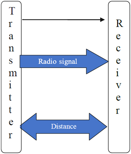
- ToA: It finds the distance and time at which the incoming signal is received, as the speed of propagation information is already available. Both the transmitter and the receiver end are synchronized and the start time of transmission is known. The parameter c (speed of the light) is known and distance calculation is done, based on the time of the incoming signal’s arrival at the receiver end [15, 16]. In this method, synchronization must be required between the transmitter and the receiver clocks for accuracy, which leads to additional hardware requirements at both units, and increases complexity. Fig. 1.1 illustrates the concept of ToA.
- TDoA: In this scheme, the medium used for transmission gives a different speed. As shown in Fig. 1.2, the radio and the ultrasound signals are transmitted from the transmitter end. The arrival of any signal at the receiver end is used to measure the arrival of the other signal. The distance is calculated based on the arrival time of these two transmitted signals. This method provides accuracy under line of sight (LOS) conditions but, if certain disturbances occur in the environmental conditions, it leads to the failure of LOS conditions. Also, with the change in environmental conditions, these arrival times are going to vary from their actual values which leads to incorrect distance measurements.
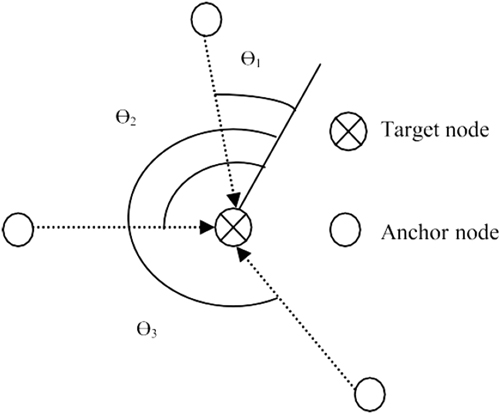
- Angle of Arrival (AoA): The distance calculation between the anchor and the target nodes is also calculated using the Angle of Arrival method. In this method, an angle is made between the two lines, where the first line connects the transmitting and receiving ends and second line is between the receiver and the other direction, taken as a reference, as shown in Fig. 1.3. The distance measured through this technique is more accurate than the distance calculated using the RSSI method mentioned above [17].
- Proximity: This is the simplest and cheapest method available for calculating the distance between the nodes because it measures distances only between those nodes which are inter-connected and within range. The hardware configuration required is simplest under this scheme [18].
- Picture Analysis: This technique behaves in a different manner from the above-mentioned techniques. In this, the distance calculations are carried out using a picture or on the basis of scene analysis. In this technique, additional hardware is required which leads to complexity and is the main drawback of this technique.


1.2.2 Computational Stage
In the second, computational stage, the estimations done on determining the distance and angles in the previous stage are collated for calculating the positions of the unknown nodes. These methods, which work on computational analysis, are discussed as follows.
- Trilateration: In this scheme the estimated coordinates of the target node is determined with the help of three anchor nodes, and the location of the tracking nodes is calculated [19]. As shown in Fig. 1.4, the determination of the target nodes coordinates is obtained from the coincidence of consecutive circles. In the case of determining the 2-D coordinates, at least three anchor nodes are required.
- Triangulation: Geometrically, the triangulation technique is used to obtain the information of 2-D coordinates on the basis of angles calculated between the nodes and the reference points. By using mathematical sine and cosine rules, the position of the target nodes can be calculated [20]. Fig. 1.5 shows this technique.
- Multilateration: In the trilateration approach, the calculated distance is not perfect because the joining of the three circles does not correspond to a single point. In order to cope with this limitation, at least three anchor nodes are required, a process termed multilateration [21]. The results of this technique are much more efficient than those from trilateration. Fig. 1.6 represents this concept.


Three anchor nodes are assumed with their known position, i.e., (x i, y i) for i = 1,2,3 and the unknown position of the target nodes (x t, y t) is calculated by using the equation as given:
|
|
(1.3) |
where d i,t represents the distance between the target nodes and the anchor nodes.
1.3 Classification of Localization Algorithms Available in WSNs
The localization concept in sensor networks is gaining importance in almost all real-world applications of WSNs. The survey of these types of algorithms provides detailed explanations of the different techniques available for localizing the nodes referred to as anchor-based, anchor-free, range-free and range-based nodes, etc. Every node connected within the network transmits a beacon signal, that will be analyzed by the receiver at the receiver section in order to measure the range, which will help in counting the number of hops. Fig. 1.7 classifies the various available localization algorithms.

1.3.1 Localization Based on Hop Counts
In single-hop localizations, the unknown nodes, called target nodes, are localized in that they are only one hop away from the known positions of the anchor nodes, whereas, in the case of multiple hop schemes, the unknown nodes and the known anchor nodes are more than one hop count apart; multiple hop counts are those which connect the two nodes. The methods used for single-hop counts are Angle of Arrival, Time of Arrival, Time Difference of Arrival, and Received Signal Strength Indicator, whereas the multi-hop method covers Distance Vector Hopping scheme, Approximation of Points Residing in the Triangles, and Multidimensional Scaling. Fig. 1.8 represents this concept. In these methods, additional numbers of anchor nodes are required, which is the major drawback [22 –25].

A matrix, symmetric in nature, is applied as an input to the multi-hop WSN localization method. In this, hop counts on the basis of distance between the nodes are calculated and used. The techniques used under this scheme are referred to as range-based and range-free localizations.
1.3.2 Localization Based on Range-based and Range-free Techniques
Localization algorithms are divided into two categories, namely range-based and range-free techniques. In range-based localization techniques, the anchor node’s range information is required, but, in the second method, information relevant to range is not required. By using some specialized hardware, the distances between the nodes is calculated precisely. The main issue arising from this technique is accuracy degradation taking place in case of mobility scenario and of various noises taking place in the environment.
A network formation in the case of the range-free technique is that in which the hop count is directly proportional to the distance between them. In case of range-free techniques, the coordinates are calculated on the basis of radio connectivity information among their available neighboring nodes. This technique is more efficient, in terms of simplicity and cost- effectiveness, than the range-based localization techniques. Several approaches related to range-free techniques are given below [26, 27].
- 1. Based on the Centroid method: This method was developed by Blusu et al. [28]. In this algorithm, at least three anchor nodes are required in order to locate the position of the unknown node, which are in its neighborhood position. Eq. (1.4) represents the method of calculating the centroid, where
-
(1.4) - 2. DV-Hop method: In the DV-Hop method, the hop count between two anchor nodes is calculated and, from this information obtained, the length of each hop is calculated. The information gathered by every anchor node is floated or shared into the sensing field area. This information will help locate the target nodes by estimating the multi-hop range [26, 29, 30].
- 3. Approximating Point in Triangular method (APIT): In this technique, the area under investigation is segregated into triangular regions. A node lying near or far from the triangular region resides in the corresponding triangle by narrowing down its area [11].
- 4. Multi-dimensional scaling (MDS): In this method, again on the basis of distance, all nodes will maintain a distance matrix. After estimating the distance matrix, Dijkstra’s algorithm for finding the shortest path is used to design a complete matrix. When the observation accuracy of a sensor becomes worse, this technique is not efficient during that time, then a hybrid technique, in which this method is used in combination with trilateration, can provide the efficient results [31].
1.3.3 Localization Based on Anchor-based and Anchor-free Techniques
These are the two techniques available on which the location of unknown nodes is relied upon. In the first (anchor-based) method, the information on the anchor node is required in order to calculate the coordinates of the unknown node; in the case of anchor-free techniques, no such information about the anchor is required. In the deployment stage the position of a few nodes, known as anchor nodes, are known, as they include a GPS feature, whereas, in the case of the anchor-free method, localization is achieved, using the information of the relative coordinates [32, 33]. The main motive behind the use of anchor-based method is the calculation of the distance from the unknown nodes to the known nodes; after the calculation on this basis is carried out between them, then, by using localization algorithms, the unknown node determines its coordinates in space, as, for determining 2-D coordinates, at least three anchor nodes are required and, for determining 3-D coordinates, four anchor nodes at least are required.
In cases where no anchor node is available, there are two important steps to be followed for determining or localizing the unknown nodes.
By the use of different localization methods available, every node in the sensing field computes the distance between them and their neighboring nodes.
Then, on the basis of distance, every node in the sensing field determines its coordinates itself.
1.3.4 Centralized and Distributed Localization
A central processor is responsible for computing all the computations by the centralized method, but, in the latter method, the computations are performed using the inner sensor measurements. The main advantage of using the centralized method is that each node does not need to perform the computations. The major drawback of using this technique is that all the nodes send their data back to the base station. Simulated annealing and RSSI-based localization come under the classification of centralized localization algorithms. These algorithms are better in terms of localization accuracy because complete information about the connectivity and distance is available between the deployed sensor nodes and their neighbors [34].
In the case of distributed localization algorithms, the sensors deployed in the field compute the required information in terms of either connectivity or distance on an individual basis. In this method, each node communicates with them or with their neighbors, in order to determine their own position in the network. Beacon-based, coordinate system-based and hybrid localizations are some of the examples of distributed localization algorithms. In this method, many iterations are required to achieve stability, resulting in the technique being a little slow, which leads to a drawback of this method [35].
1.3.5 Static and Dynamic Localization
In the static algorithms, once the nodes are deployed in the region of interest, they will not move; the dynamic method nodes deployed in the sensing field have some mobility and will move accordingly [36 –38]. In static algorithms, the coordinates of unknown nodes are determined during the set-up of static WSNs. But in the case of the dynamic method, a continuous tracking of sensor nodes is required as they are moving and changing their coordinate values. A little extra time is required to determine the coordinates of the moving nodes; for tracking the position of moving nodes, a fast localization feature is required, using this procedure. In the case of static algorithms, the convergence rate is fast. There are many range-based techniques available, like approximate point in triangulation and lateration, multilateration, and the modified centroid method, which are some of the static localization techniques.
It is very difficult to track the location of moving target nodes because it has to be determined periodically. There are various techniques available in the literature, of which the Kalman filter is one which works well in noisy environments. Road navigation in the absence of GPS features is a property of Kalman Filters [39, 40]. In order to predict the system’s future states, the Kalman filter is one of the useful techniques.
These issues are described in the following section.
1.4 Localization Challenges
In many real-time applications, the localization concept is becoming an important and essential requirement in the field of WSN. The available literature presents many challenges to be faced, while using the concepts of localization [1]. As represented in Fig. 1.9, there are some issues that need to be taken care of in order to improve the localization process of the WSNs.

1.4.1 Energy of the node
The sensor nodes deployed in the sensing field in the area of WSNs have non-replaceable and limited-energy battery units for performing the operations, such as sensing and reporting. The whole system becomes worse if special care is not taken with regard to battery units. A lot of research has been conducted in order to improve the energy of the node [41].
1.4.2 Node Mobility
In order to maintain the node’s connectivity in the mobility scenario is quite a challenging task in localization. In the case of static WSNs, the node, once estimated, is not going to change its position as it is fixed, but, in the case of dynamic WSNs, the nodes periodically shift from one position to another position, and the deployed sensor node has to determine and estimate the position periodically [36, 38]. So, localization is becoming a major source of interest amongst researchers.
1.4.3 Transmission Range of Node
In most of the localization techniques, a beacon signal is required for determining the locations of unknown nodes. Beacon nodes are equipped with a GPS feature which helps these nodes to be placed at a position with known coordinates, and, with this feature, one can obtain a proper connectivity in between the beacon and the target nodes. So, the transmission range of a node plays a key role in estimating the locations of unknown nodes.
1.4.4 Localization Security
As in WSNs, most of the times this set-up is installed in unfriendly locations. Some of the problems that occur in localization are overshadowing and distance away from attack [42]. So, researchers are showing interest in improving the security of localization.
1.4.5 Localization Accuracy
Accuracy is determined by calculating the difference between the actual and the estimated position of the sensor node. It is a difficult task to obtain the accurate location of the sensor node by applying localization algorithms. So, by using available or new localization algorithms, it is possible to obtain optimum results [43, 44].
1.4.6 Multi-Dimensional Localization
Basically, in order to obtain the coordinates of unknown nodes (target nodes), localization algorithms are used. Some of the applications require knowledge of 2D and 3D coordinates [36].
1.5 Determination of the 2-D and 3-D Coordinates of the Sensor Node
As many advances and improvements in the field of wireless communication have taken place in recent years, this has encouraged the use of WSNs in many real-world applications. Localization of sensor nodes becomes necessary in almost every application in WSNs. There are various localization algorithms available in the literature, which will determine the location of target nodes placed in the sensing field, which, in turn, are possible with or without the use of anchor nodes.
1.5.1 Determination of 2-D Coordinates
Bulusu et al. [28], in their research, investigated localization in outdoor conditions without using GPS features. They used the centroid method for calculating the coordinates of the unknown nodes. Lee et al. [45] represented their work on localization by using very few anchors in the field. Their work presented and claimed a higher accuracy in estimating the distance by finding the shortest path. Awad et al. [46] presented two ways for estimating the distance; the first way was to use the available statistical methods and the other one was to use the concepts of neural networks for computing the distance. Their conclusions were based on the parameters which degrade the quality of distance measurements, such as transmitted power, RF frequencies, mobility of nodes, and localization algorithms. Savvides et al. [47], in their work, discussed the use of the multilateration technique. The authors presented a distributive approach in that sensor nodes were collectively going to solve an optimization problem, which a single sensor could not solve. Three state problems are discussed in this paper. In state-1, a combined approach was taken, the second state represents the computation of starting estimates, and, in the final state, again, reframing of positions was carried out. Savvides et al. [48] presented an approach to localizing sensors in a temporary network that allows the deployed sensors in the field to find their locations using distributive methods. Although location estimates are more accurate by using centralized methods, by using a distributive approach, the system is more robust and will result in an effective distribution of power consumption in the network. Sumathi and Srinivasan [49] used the least squares method for estimating the locations of static target nodes by the use of single anchor nodes, on the basis of RSSI measurements.
Guo et al. [50] presented a different approach in which there is no relation or mapping of estimating distances based on RSSI values, using the method named as the Perpendicular Intersection method. Using this geometric relationship, the positions of the nodes are computed. Kim and Lee [51] presented a localization technique that is range based and in which the movement of the mobile anchor node is based on some strategy, known as MBAL (Mobile Beacon-Assisted Localization). Their scheme provided the best selection of the path, with fewer complexities.
In their conclusions, Karim et al. [52] discussed the range-free techniques that are efficient in terms of energy with the use of fewer anchor nodes. They claimed that their technique is less complex and more accurate by using very few anchor nodes. Li et al. [53] proposed a method that provides efficient and robust localization in real-time scenarios. The techniques used are named the Breadth-First (BRF) and Backtracking Greedy (BTG) algorithms. Chen et al. [54] presented an approach that is classified under the range-free methods. Their work stated that their scheme is simple and practical, in which a comparison among the nodes is based on RSSI values and this consumes much less energy and shows great accuracy, while using the concepts of mobile anchors. Khelifi et al. [55] proposed two different localization algorithms, namely time-driven and event-driven for mobile WSNs. Stone and Camp [56] discussed the localization algorithms that use the information of anchors, and computed the performance and accuracy of localization relative to anchor mobility and target nodes. There is much more research which we have not mentioned, and conclusions are available in the literature [57 –63].
1.5.2 Determination of 3-D Coordinates
Shi et al. [64] presented Ultra-Wide Band, a Time of Arrival method determining the 3-D coordinates required for localization. They discussed that distance calculation, using their technique between the anchor node and the unknown node, can be more precise than other techniques. Wang et al. [65] presented a scheme based on the Distance Vector hopping algorithm, that can localize 3-D coordinates of a sensor node more precisely and effectively, but its complexity and huge deployment cost are its major limitations. Xu et al. [66] discussed a hybrid method by using Distance Vector hopping combined with the Newton method for optimization. The authors considered two parameters, one of which is coverage and the other accuracy, for their proposed algorithm. Li et al. [67] developed a model for determining 3-D coordinates in a WSN environment on the basis of the RSSI model. They proposed a model for obtaining relevance between the Degree of Irregularity and variation in the ranges of the transmitted signal. Ahmad et al. [68] developed an algorithm for the determination of 3-D coordinates, using a parametric method. In their algorithm, very few anchor nodes are available for localization and will provide better results because the network is shrinking towards a common point known as the central point. Zhang et al. [69] proposed a localization algorithm that depended upon an expensive beacon signal. MDS-MAP, DVHOP, and the Centroid method are methods modified from 2-D coordinates to 3-D coordinates, which are available in the literature [71 –75]. In obtaining the 3-D coordinates in applications deployed in an underwater network [76], Cheng et al. [77], and Zhou et al. [78] surveyed this application. In these methods, localization is achieved using information based on connectivity and the number of anchors. Tomic et al. [79] presented a hybrid method in developing 3-D WSNs. In this scheme, an estimate on the basis of least squares criterion is used. Chan et al. [80] proposed a method for solving a problem based on transmission power as some 3-D localization methods require specific directional information, by implementing a directional antenna on anchor nodes [81, 82].
1.6 Applications
Navigational services are now being used by everyone everywhere in the world, but accurate positioning of mobile devices is becoming a current research topic.
1.6.1 Services Based on Location
Through mobile networks and/or the internet, the information about the location is provided to end users. Applications based on navigational services can provide the connectivity to link the position of the mobile user, with geographical locations tracked by mobile users. These services are essential in both indoor and outdoor environments. These types of services are required for guiding the users to a particular area of interest. Also, they are used in a public place, e.g., in railway stations or bus stations, to direct the passengers to a particular desired place.
1.6.2 Health and Smart Living Applications
Localization in the indoor environments plays a great role for these types of applications. These types of applications are helpful for determining and monitoring the health of elderly people [83].
1.6.3 Robotics
Robotics is one of the important applications in the field of localization. There is much research going on for the development of these types of applications. The cooperation between the installed robots in the field is required for certain applications like surveillance and for the tracking of other unknown areas [84].
1.6.4 Cellular Technology
Many challenges and issues about the accurate determination of location are determined by cellular technology [85], as the growth in the mobile generation leads to an improvement in the accuracy.
1.7 Techniques Used to Improve Localization
1.7.1 Features of Optimization Techniques
The features of optimization techniques are listed below.
1.7.1.1 Speed
In real-time environments, the convergence rate of the localization algorithm used should be fast enough.
1.7.1.2 Adaptability
The system should adapt to the environment and report accordingly, in case the node fails.
1.7.1.3 Self-Organizing Capability
The system will have self-organizing capabilities, meaning that, in cases of mobility, it will re-organize the network itself. Some pre-defined rules and instructions are posed on the network, so that system will adapt the changes accordingly.
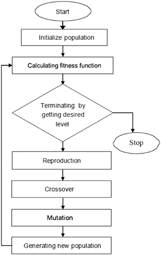
1.7.2 Genetic Algorithms (GA)
This is a technique based on search and optimization and is used for finding the estimated results. It begins its search with random solutions and these solutions are assigned a fitness function that is relative to their objective function. Then, a set of new populations is formed by using three genetic operators, named as reproduction, cross-over and mutation [86]. An iterative operation in GA takes place using all three operators until a terminated criterion is not reached. For decades, GA has been used in a wide variety of applications, because of its simplicity. The basic flow of genetic algorithms is given in Fig. 1.10.
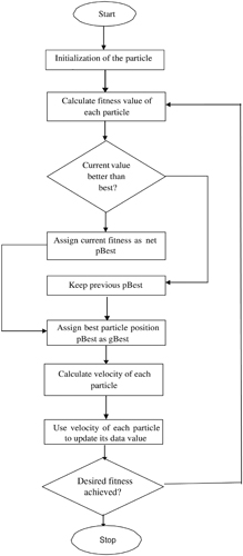
1.7.3 Particle Swarm Optimization (PSO)
A technique developed by Kennedy and Eberhart is known as PSO [87], based on the behavior of birds. It is an efficient algorithm and its implementation stage is easier. A random number of particles is deployed in the search space and the objective function is calculated accordingly. Then, the movement is applied to the particles deployed in the search space [88]. A particle moving in the search space collects ‘pbest’ and ‘gbest’ positions in the space. The idea is illustrated in Fig. 1.11.
1.7.4 Biogeography Based Optimization (BBO)
In BBO, the term HIS (Habitat Suitability Index) represents the fitness function. The higher the value of HIS, the better the place is for the species to live, whereas lower HIS values indicate an inappropriate place for the species to live. The basic idea about the BBO algorithm is shown in Fig. 1.12.

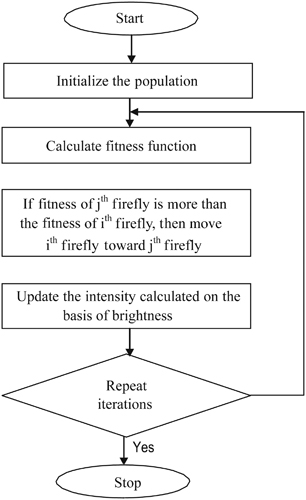
1.7.5 Firefly Algorithm
The firefly algorithm was proposed by Yang [89]. The behavior of fireflies is used in this algorithm and the rules followed by the fireflies are as follows:
- All fireflies are unisex as they move from one place to another notwithstanding of sex [90].
- The parameter which attracts the fireflies towards each other is attractiveness, which is directly proportional to the glowing nature of the fireflies, and, as they move a certain distance apart, their brightness is reduced. So, fireflies will not follow each other in that particular case. If there is no brighter firefly found, then this event is random in nature. The fitness function in this case is represented by the glowing nature of fireflies. Then, according to these rules, the firefly algorithm is represented in Fig. 1.13.
According to the Free Lunch theory, no single algorithm is best-suited to each optimization problem. There are many more types of optimization algorithms that are reported in the literature, which can be applied to localization problems to check their performance.
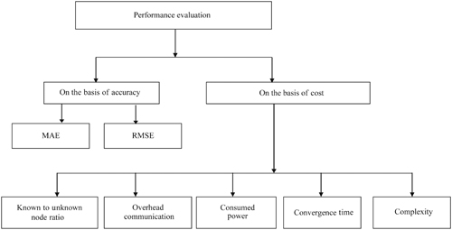
1.8 Criteria for Evaluation and Performance Parameters
In WSNs, multiple errors occur, such as errors due to range problems, errors due to non-availability of GPS signals and sometimes localization algorithms, which are used for certain applications, degrade the accuracy of the system. Range error arises due to incorrect measurements carried out on the basis of distances. Similarly, errors in anchor position lead to a GPS error. There are certain parameters on which the performance of the algorithms depends on accuracy in terms of location, its cost and coverage. The evaluation procedure is described in Fig. 1.14.
- Accuracy in Location: In this, the difference between the node’s original position and the estimated position is calculated using any localization algorithm and the difference between the two leads to an error. By using this information, the determination of the accuracy parameter is calculated; the smaller the error, the greater will be the accuracy, and vice versa.
- Flexibility to Error and Noise: The localization algorithm chosen for the determination of location should be flexible enough to combat errors or noises originating from the input side.
- Coverage: The coverage parameter depends upon a few conditions, such as the number of anchor nodes deployed in the sensing field. The larger the number, the better the coverage.
- Cost: In this, the cost parameter is evaluated on the basis of power consumed and the time taken by the algorithms to localize the nodes, so that communication between the nodes can be initiated.
1.8.1 Parameter Calculations on the Basis of Accuracy
The accuracy term is used to match the positions of the actual and the estimated target nodes. The difference between the two positions leads to errors and these errors are named the Mean Absolute Error and the Root Mean Square Error.
Mean Absolute Error (MAE): MAE is basically calculated with respect to the continuous variables and it is an important parameter for finding out the accuracy of a localization algorithm used in a specified application. The equation for MAE is Eq. (1.5), where (x t, y t, z t) is the current position, (x e, y e, z e) is the calculated position, and N t represents the total number of sensor nodes deployed.
|
|
(1.5) |
Root Mean Square Error (RMSE): This parameter also represents a measure of accuracy and is given by Eq. (1.6),
|
|
(1.6) |
1.8.2 Evaluation on the basis of cost metrics
In almost every application, cost factor determination plays an important role. In the context of localization, the parameters which contribute to the cost are power consumed during the set-up stage, how many anchor nodes are required for this process, and the total time required to localize all the nodes in the network. If lifetime enhancement of the network is important at the same time, cost management also plays an equal role. There is a trade-off between these two. The ratio of known positions of the anchor nodes to the unknown positions, power consumed, and time taken by the localization algorithm to localize all the nodes play important roles in determining cost metrics.
- Anchor to Target Ratio: In terms of cost metrics, anchor nodes are the ones which are deployed in the sensing field with GPS features enabled in them. In order to save the cost, we need to install only a few anchor nodes in the field as they are expensive, and, in order to localize the target nodes, this terminology is used. It is defined as the number of anchor nodes required to localize the target nodes.
- Overhead during Communication: As the number of sensor nodes deployed in the sensor field increases, the communication overhead also increases to a greater extent. The overhead can be calculated by finding out the total number of packets sent.
- Convergence Time: The time taken by the localization algorithm to collect all the information regarding localizing all the nodes present in the network represents the convergence time. As the network size increases, this parameter is affected.
- Algorithmic Complexity: Algorithmic complexity is always defined with some standard notions (O), where the higher the order, like O(n 3) and O(n 2), the longer time it will take to converge, with this parameter representing the complexity.
- Power Consumed: This parameter is important in terms of cost as it calculates the power consumed in a localization process.
1.9 Conclusions
In this chapter, the two different scenarios, the Static and Dynamic issues of WSNs, are discussed. There are two main stages on which estimation of a sensor node’s location depends, i.e., the measurement stage and the computational stage. Furthermore, they are classified on the basis of range based or range free, anchor based or anchor free, and the mobility scenario has already been discussed. There are certain challenges faced in the localization process. The major challenge is to localize the sensor node’s location in 2-D and 3-D scenarios. Many optimization techniques have been used to estimate the accurate locations of the sensor nodes. Still, there are open questions in this research area, like the localization in mobility-based scenarios and the use of smaller numbers of anchor nodes to save costs. Therefore, one can introduce different optimization techniques in the future to solve the various issues arising in the localization process.
Bibliography
- 1. Karl, H, Willig, A (2007) Protocols and Architectures for Wireless Sensor Networks. John Wiley & Sons.
- 2. Cheng, L, Wu, C D Zhang Indoor robot localization based on wireless sensor networks. IEEE Trans. Consum. Electron. 57(3), 1099–1104.
- 3. Barsocchi, P, Lenzi, S, Chessa, S, Giunta G (2009) A novel approach to indoor RSSI localization by automatic calibration of the wireless propagation model. In: IEEE 69th Vehicular Technology Conference, pp. 1–5, VTC Spring.
- 4. Chan, Y T, Tsui, W Y, So, H C Ching (2006) Time-of-arrival based localization under NLOS conditions. IEEE Trans. Veh. Technol. 55(1), 17–24.
- 5. Xu, E Ding, Dasgupta, Z (2011) Source localization in wireless sensor networks from signal time-of-arrival measurements. IEEE Trans. Sig. Process. 59(6), 2887–2897.
- 6. Gillette, M D, Silverman, H F (2008) A linear closed-form algorithm for source localization from time-differences of arrival. IEEE Sig. Process. Lett. 15, 1–4.
- 7. Rong, P Sichitiu (2006) Angle of arrival localization for wireless sensor networks. In: 3rd Annual IEEE Communications Society on Sensor and Ad Hoc Communications and Networks, SECON’06, vol. 1, pp. 374–382.
- 8. Kułakowski, P, ValesAlonso J (2010) Angle-of-arrival localization based on antenna arrays for wireless sensor networks. Comput. Electr. Eng. 36(6), 1181–1186.
- 9. Deng, B Huang, Zhang, G, Liu, L H (2008) Improved centroid localization algorithm in WSNs. In: 3rd International Conference on Intelligent System and Knowledge Engineering, ISKE 2008, vol. 1, pp. 1260–1264.
- 10. Chen, K Wang An Improved dv-Hop Localization Algorithm for Wireless Sensor Networks Hindawi.
- 11. Wang, Zeng, Jin, J H (2009) Improvement on APIT localization algorithms for wireless sensor networks. In: International Conference on Networks Security, Wireless Communications and Trusted Computing, NSWCTC’09, vol. 1, pp. 719–723.
- 12. Shang, Y, Ruml W (2004) Improved MDS-Based Localization in Twenty-Third Annual Joint Conference of the IEEE Computer and Communications Societies, Infocom, vol. 4, pp. 2640–2651.
- 13. Alippi, C, Vanini, G (2006) A RSSI-based and calibrated centralized localization technique for wireless sensor networks. In: Fourth Annual IEEE International Conference on Pervasive Computing and Communications Workshops, 2006. PerCom Workshops 2006, p. 5.
- 14. Deng Yin, Z, Guo-Dong, C (2012) A union node localization algorithm based on RSSI and DV-Hop for WSNs. In: Second International Conference on Instrumentation, Measurement, Computer, Communication and Control (IMCCC), pp. 1094–1098.
- 15. Humphrey, D, Hedley, M (2008) Super-resolution time of arrival for indoor localization. In: IEEE International Conference on Communications, pp. 3286–3290.
- 16. Cheung, K W, So, H C, Ma, W (2004) Least squares algorithms for time-of- arrival-based mobile location. IEEE Trans. Sig. Process. 52(4), 1121–1130.
- 17. Azzouzi, S, Cremer, M, Dettmar, U, Kronberger, R, Knie, T (2011) New measurement results for the localization of UHF RFID transponders using an angle of arrival (AOA) approach. In: IEEE International Conference on RFID (RFID), pp. 91–97.
- 18. Torre, A, Rallet, A (2005) Proximity and localization. Reg. Stud. 39(1), 47–59.
- 19. Boukerche, A, Oliveira, H A, Nakamura, E F, Loureiro, A A Localization systems for wireless sensor networks. IEEE Wirel. Commun. 14(6), 6930–6952.
- 20. Tekdas, O, Isler, V (2010) Sensor placement for triangulation-based localization. IEEE Trans. Automat. Sci. Eng. 7(3), 681–685.
- 21. Zhou, Y, Li, J, Lamont, L (2012) Multilateration localization in the presence of anchor location uncertainties. In: IEEE Global Communications Conference (GLOBECOM), pp. 309–314.
- 22. Bal, M, Liu, M, Shen, W, Ghenniwa, H (2009) Localization in cooperative wireless sensor networks: A review. In: 13th International Conference on Computer Supported Cooperative Work in Design, CSCWD, pp. 438–443.
- 23. Whitehouse, K, Karlof, C, Culler, D (2007) A practical evaluation of radio signal strength for ranging-based localization. ACM SIGMOBILE Mob. Comput. Commun. Rev. 11(1), 41–52.
- 24. Franceschini, F, Galetto, M, Maisano, D, Mastrogiacomo, L (2009) A review of localization algorithms for distributed wireless sensor networks in manufacturing. Int. J. Comput. Integr. Manufact. 22(7), 698–716.
- 25. Lakafosis, V, Tentzeris, M M From single-to multihop the status of wireless localization. IEEE Microw. Mag. 10(7), 34–41.
- 26. He, T, Huang, C, Blum, B M, Stankovic, J A, Abdelzaher, T (2003) Range-free localization schemes for large scale sensor networks. In: Proceedings of the 9th Annual International Conference on Mobile Computing and Networking, pp. 81–95.
- 27. Dil, B, Dulman, S, Havinga, P (2006) Range-based localization in mobile sensor networks. Wirel. Sensor Netw. 0302-9743, 164–179.
- 28. Bulusu, N, Heidemann, J, Estrin, D (2000) GPS-less low-cost outdoor localization for very small devices. IEEE Pers. Commun. 7(5), 28–34.
- 29. Kumar, S, Lobiyal, D (2013) An advanced DV-Hop localization algorithm for wireless sensor networks. Wirel. Pers. Commun. 71, 1–21.
- 30. Tian, S, Zhang, X, Liu, P, Sun, P, Wang, X (2007) A RSSI-based DV-Hop algorithm for wireless sensor networks. In: International Conference on Wireless Communications, Networking and Mobile Computing, WiCom, pp. 2555–2558.
- 31. Stojkoska, B R, Kirandziska (2013) Improved MDS-based algorithm for nodes localization in wireless sensor networks. In: EUROCON 2013 IEEE, pp. 608–613.
- 32. Priyantha, N B, Balakrishnan, H, Demaine, E Teller (2003) Anchor-free distributed localization in sensor networks. In: Proceedings of the 1st International Conference on Embedded Networked Sensor Systems, pp. 340–341.
- 33. Ssu, K F, Ou, C H, Jiau, H C (2005) Localization with mobile anchor points in wireless sensor networks. IEEE Trans. Veh. Technol. 54(3), 1187–1197.
- 34. Zhang, Q Huang, Wang, J, Jin, J, Ye, C, Zhang, J W (2008) A new centralized localization algorithm for wireless sensor network. In: Third International Conference on Communications and Networking in China, 2008. ChinaCom 2008, pp. 625–629.
- 35. Langendoen, K, Reijers, N (2003) Distributed localization in wireless sensor networks: A quantitative comparison. Comput. Netw. 43(4), 499–518.
- 36. Singh, P, Khosla, A Kumar A Khosla 3d localization of moving target nodes using single anchor node in anisotropic wireless sensor networks. AEU Int. J. Electron. Commun. 82, 543–552.
- 37. Parulpreet, S Arun, Anil, K, Mamta, K (2017) Wireless sensor network localization and its location optimization using bio inspired localization algorithm: A survey. Int. J. Curr. Eng. Sci. Res. 10(4), 74–80.
- 38. Singh, P, Khosla, A Kumar, Khosla, A (2017) A novel approach for localization of moving target nodes in wireless sensor networks. Int. J. Grid Distrib. Comput. 10(10), 33–44.
- 39. Roumeliotis, S I, Bekey, G A (2000) Bayesian estimation and Kalman filtering: A unified framework for mobile robot localization. In: IEEE International Conference on Robotics and Automation, vol. 3, pp. 2985–2992.
- 40. Reina, G, Vargas, A, Nagatani, K Yoshida (2007) Adaptive Kalman filtering for GPS-based mobile robot localization. In: IEEE International Workshop on Safety, Security and Rescue Robotics (SSRR), pp. 1–6.
- 41. Patwari, N, Ash, J N (2005) Locating the nodes cooperative localization in wireless sensor networks. IEEE Sig. Process. Mag. 22(4), 54–69.
- 42. Jiang, J, Han, G, Zhu, C Dong, Zhang, Y (2011) Secure localization in wireless sensor networks: A survey. JCM 6(6), 460–470.
- 43. Kumar, A, Khosla, A, Saini, J S Singh (2012) Meta-heuristic range based node localization algorithm for wireless sensor networks. In: International Conference on Localization and GNSS (ICL-GNSS), pp. 1–7.
- 44. Kumar, A, Khosla, A, Saini, J S, Sidhu (2015) Range-free 3d node localization in anisotropic wireless sensor networks. Appl. Soft Comput. 34, 438–448.
- 45. Lee, S, Park, C, Lee, M J, Kim S (2014) Multihop range-free localization with approximate shortest path in anisotropic wireless sensor networks. EURASIP J. Wirel. Commun. Netw. 1, 1–12.
- 46. Awad, A, Frunzke, T, Dressler F (2007) Adaptive distance estimation and localization in WSN using RSSI measures. In: 10th Euromicro Conference on Digital System Design Architectures, Methods and Tools, pp. 471–478.
- 47. Savvides, A, Park, H Srivastava, M B (2002) The bits and flops of the n-hop multilateration primitive for node localization problems. In: Proceedings of the 1st ACM International Workshop on Wireless Sensor Networks and Applications, pp. 112–121.
- 48. Savvides, A, Han, C C, Shrivastava (2001) Dynamic fine-grained localization in ad-hoc networks of sensors. In: 7th Annual International Conference on Mobile Computing and Networking, pp. 166–179.
- 49. Sumathi, R, Srinivasan, R (2011) RSS-based location estimation in mobility assisted wireless sensor networks. In: 6th International Conference on Intelligent Data Acquisition and Advanced Computing Systems (IDAACS), vol. 2, pp. 848–852.
- 50. Guo, Z, Guo, Y Hong, Jin, F, Feng, Y, Liu, Y, Feng, Y, Liu, Y (2010) Perpendicular intersection: Locating wireless sensors with mobile beacon. IEEE Trans. Veh. Technol. 59(7), 3501–3509.
- 51. Kim, K, Lee, W M B A L (2007) a mobile beacon-assisted localization scheme for wireless sensor networks. In: 16th International Conference on Computer Communications and Networks, pp. 57–62.
- 52. Karim, L Nasser, El Salti, N (2010) RELMA: A range free localization approach using mobile anchor node for wireless sensor networks. In: IEEE IEEE Global Telecommunications Conference (GLOBECOM 2010), pp. 1–5.
- 53. Li, H Wang, Li, J X H (2008) Real-time path planning of mobile anchor node in localization for wireless sensor networks. In: International Conference on Information and Automation, pp. 384–389.
- 54. Chen, Y S, Ting, Y J, Ke, C H, Chilamkruti, N, Park, J H (2013) Efficient localization scheme with ring overlapping by utilizing mobile anchors in wireless sensor networks. ACM Trans. Embedded Comput. Syst. (TECS) 12(2), 20.
- 55. Khelifi, M, Benyahia, I, Moussaoui, S, Abdesselam, Naït (2015) An overview of localization algorithms in mobile wireless sensor networks. In: International Conference on Protocol Engineering (ICPE) and International Conference on New Technologies of Distributed Systems (NTDS), pp. 1–6.
- 56. Stone, K, Camp, T (2012) A survey of distance-based wireless sensor network localization techniques. Int. J. Pervasive Comput. Commun. 8(2), 158–183.
- 57. Huang, S C, Chang, H Y (2015) A farmland multimedia data collection method using mobile sink for wireless sensor networks. Multimedia Tool. Appl. 2015, 1–16.
- 58. Gholami, M, Cai, N, Brennan, R (2013) An artificial neural network approach to the problem of wireless sensors network localization. Robot. Comput. Integr. Manufact. 29(1), 96–109.
- 59. Singh, P, Saini, H S (2015) Average localization accuracy in mobile wireless sensor networks. J. Mob. Syst. Appl. Serv. 1(2), 77–81.
- 60. Wang, J, Han, T (2011) A self-adapting dynamic localization algorithm for mobile nodes in wireless sensor networks. Procedia Environ. Sci. 11, 270–274.
- 61. Ding, Y Wang, Xiao, C L (2010) Using mobile beacons to locate sensors in obstructed environments. J. Parallel Distrib. Comput. 70(6), 644–656.
- 62. Chen, H, Gao, F, Martins, M Huang, Liang, P J (2013) Accurate and efficient node localization for mobile sensor networks. Mob. Netw. Appl. 18(1), 141–147.
- 63. Wang, Y, Wang, Z (2011) Accurate and computation-efficient localization for mobile sensor networks. In: International Conference on Wireless Communications and Signal Processing (WCSP), pp. 1–5.
- 64. Shi, Q, Huo, H, Fang, T, Li, D (2009) A 3d node localization scheme for wireless sensor networks. IEICE Electron. Express 6(3), 167–172.
- 65. Wang, L Zhang, Cao, J D (2012) A new 3-dimensional DV-Hop localization algorithm. J. Comput. Inf. Syst. 8(6), 2463–2475.
- 66. Xu, Y Zhuang, Gu, Y J J An improved 3d localization algorithm for the wireless sensor network.
- 67. Li, J Zhong, Lu, X I T (2014) Three-dimensional node localization algorithm for WSN based on differential RSS irregular transmission model. J. Commun. 9(5), 391–397.
- 68. Ahmad, T, Li, X J, Seet, B C (2017) Parametric loop division for 3d localization in wireless sensor networks. Sensors 17(7), 1697.
- 69. Zhang, L Zhou, Cheng, X Q (2006) Landscape-3d; a robust localization scheme for sensor networks over complex 3d terrains. In: Proceedings of the 31st IEEE Conference on Local Computer Networks, pp. 239–246.
- 70. Tan, G Jiang, Zhang, H, Yin, S, Kermarrec, Z, AM (2013) Connectivity-based and anchor-free localization in large-scale 2d/3d sensor networks. ACM Trans. Sens. Netw. (TOSN) 10(1), 6.
- 71. Peng, L J, Li, W W (2014) CCDC) The improvement of 3d wireless sensor network nodes localization. In: The 26th Chinese Control and Decision Conference, pp. 4873–4878.
- 72. Zhang, B, Fan, J, Dai, G, Luan, T H A hybrid localization approach in 3d wireless sensor network. Int. J. Distrib. Sens. Network 2015, 1–11.
- 73. Yu, G, Yu, F, Feng, L (2008) A three dimensional localization algorithm using a mobile anchor node under wireless channel. In: IEEE International Joint Conference on Neural Networks (IEEE World Congress on Computational Intelligence), pp. 477–483.
- 74. Liu, L Zhang, Shu, H, Chen, J (2011) A RSSI-weighted refinement method of IAPIT-3d. In: International Conference on Computer Science and Network Technology (ICCSNT), vol. 3, pp. 1973–1977.
- 75. Achanta, H K, Dasgupta, S (2012) Ding Optimum sensor placement for localization in three dimensional under log normal shadowing. In: 5th International Congress on Image and Signal Processing (CISP), pp. 1898–1901. IEEE.
- 76. Teymorian, A Y, Cheng, W, Ma, L, Cheng, X, Lu, X 3d underwater sensor network localization.
- 77. Cheng, W, Teymorian, A Y, Cheng, Ma L, Lu, X, Lu, X Z (2008) Underwater localization in sparse 3d acoustic sensor networks. In: INFOCOM 2008. The 27th Conference on Computer Communications, pp. 236–240. IEEE.
- 78. Zhou, Z, Cui, J H, Zhou, S (2007) Localization for large-scale underwater sensor networks, Networking 2007. In: Ad hoc and Sensor Networks, Wireless Networks, Next Generation Internet, pp. 108–119.
- 79. Tomic, S, Beko, M, Dinis (2017) 3-d target localization in wireless sensor networks using RSS and AOA measurements. IEEE Trans. Veh. Technol. 66(4), 3197–3210.
- 80. Chan, Y T Chan, Read, F, Jackson, W, Lee, B R (2014) Hybrid localization of an emitter by combining angle-of-arrival and received signal strength measurements. In: IEEE 27th Canadian Conference on Electrical and Computer Engineering (CCECE), pp. 1–5.
- 81. Xiang, Z, Ozguner, U (2005) A 3d positioning system for off-road autonomous vehicles. In: IEEE Intelligent Vehicles Symposium Proceedings, 130–135.
- 82. Yu, K 3-d localization error analysis in wireless networks. The IEEE Transactions on Wireless Communications 6(10), 3473–3481.
- 83. Tarrío, P, Besada, J A, Casar, J R (9–12 July 2013) Fusion of RSS and inertial measurements for calibration-free indoor pedestrian tracking. In: Proceedings of the 16th International Conference on Information Fusion, Istanbul, Turkey, pp. 1458–1464.
- 84. Wang, H, Lenz, H, Szabo, A, Bamberger, J, Hanebeck, U D (2007) WLAN-Based Pedestrian Tracking Using Particle Filters and Low-Cost MEMS Sensors, pp. 1–7.
- 85. Woodman, O, Harle, R (21–24 September 2008) Pedestrian localization for indoor environments. In: Proceedings of the International Conference on Ubiquitous Computing (UbiComp ’08), New York, NY, pp. 114–123.
- 86. Shu, J Zhang, Liu, R, Wu, L, Zhou, Z, Zhou, Z (2009) Cluster-based three-dimensional localization algorithm for large scale wireless sensor networks. JCP 4(7), 585–592.
- 87. Kennedy, J (2011) Particle Swarm Optimization. Encyclopedia of Machine Learning, pp. 760–766, Springer.
- 88. Zhang, X Wang, Fang, T J (2014) A node localization approach using particle swarm optimization in wireless sensor networks. In: International Conference on Identification, Information and Knowledge in the Internet of Things (IIKI), pp. 84–87.
- 89. Yang, X S (2009) Firefly algorithms for multimodal optimization. In: International Symposium on Stochastic Algorithms, pp. 169–178, Springer.
- 90. Harikrishnan, R, Kumar, V J S, Ponmalar, P S (2016) Firefly algorithm approach for localization in wireless sensor networks. In: 3rd International Conference on Advanced Computing, Networking and Informatics, pp. 209–214, Springer.