Faster rescue and evacuation operations in post-disaster regions are very challenging tasks, due to the uncertainty associated with localizing human beings. Additionally, failure of the pre-existing communication networks in that region prevents the trapped individuals from providing information on their location to rescuing authorities. This leads to further delays in rescue operations. The famous Brundtland Report [1] on sustainable development strongly emphasizes action on several key issues, amongst which life preservation in the face of natural disasters is one of the prominent issues.

Much importance is also given to the existing cellular network to make it stronger during such post-disaster situations, where the emphasis will be on a gradual shift from macrocell strategy in the traditional cellular network to heterogeneous topology [2]. However, this is driven by a need to increase channel capacity. With the increase in channel capacity, both data transmission speeds and number of users increases. But this tells us little about the confidence with which communication can take place under specific circumstances. Hence, under total link failure conditions, there will not be any communication, despite the capability of high data speeds and the capacity for many users per channel. The point is not to challenge the modern cellular topologies, but to emphasize the capability of heterogeneous cellular networks, specially designed for their use in disaster management. Under such circumstances, the link reliability or localization accuracy is of utmost importance, rather than data speed.

In the research investigation described in [3], emphasis was placed upon the increase in human quality-of-life for sustainable development, by using wireless sensor networks (WSNs). The work presented in [4] highlights the significance of post-disaster action planning in the context of sustainable development, where it is explained that the locals in the area should participate and ask for supply of their immediate needs and participate in decision making. However, the research work described in [5] presents the distinct types of planning schemes in the post-disaster scenario, emphasizing sustainable hazard removal rather than recovery. Likewise, the increasing need for wireless sensor networks for improved resilience post-disaster has been emphasized [6]. The author in [7] presents a detailed account of remote-sensing applications in disaster management, whereas another study focused on the need for adaptation of new methods for disaster management, including the redundancy of the rescue systems and increased communication amongst managers [8]. In [9], the authors highlighted the need to develop communication systems for disaster management. The simulation results depict that WSN will play a significant role in sustainable development where the emphasis is put on managing the post-disaster conditions. Therefore, the adoption of new methods can increase the safety factor of humans trapped in post-disaster condition.

Wireless technology plays a prominent role in disaster management and many devices have been designed that provide a warning before the disaster, thus saving the lives of individuals in disaster-prone areas [10 –12]. WSN is a very promising communication network system [13] in the field, especially where a standalone network has to be implemented in the disaster-prone area to get a pre-indication of the disaster. Also, WSN has been extensively applied in the field of environmental monitoring [14], ad-hoc vehicular networks [15], and localization of targets [16].

Localization is one of the important applications of WSN, which is of particular interest in this research area. Some of the methods for localization are listed as Global Positioning System (GPS), Angle of Arrival (AOA), Time of Arrival (TOA), Time Difference of Arrival (TDOA), and Received Signal Strength Indicator (RSSI). All of these techniques come under the category of range-based localization. RSSI-based localization is very promising in terms of the cost involved in designing the system. In this chapter, a customized mobile sensor node has been designed that focuses on RSSI-based localization. The ZigBee S2 series, integrated in the mobile sensor node, has a unique feature of sending a RSSI signal, whenever requested. Also, the cost involved for designing such nodes is minimal and, in terms of power consumption and reliability, ZigBee-based mobile sensor nodes show the best results in achieving localization. Post-disaster scenarios involve further risk to lives due to the absence of a proper responding system between those who are trapped for communication between them and the rescuing authorities, as every communication link is based on the infrastructure which is now non-operable. For localization, GPS is a mature outdoor communication technology but works inefficiently in indoor environments and has noisy access in mountainous areas. Moreover, inclusion of hardware of GPS which are cost ineffective. Unmanned aerial vehicles (UAVs) are used for real-time searching for and monitoring of individuals in disaster-prone areas [17], but they are lacking in terms of power consumption (only short flight times are possible) and accessibility at night [18, 19]. Furthermore, flight time is not enough to cover more than a limited geographical region.

The demand for WSN is centered on the capability of the node for data transmission with optimized routing algorithms. Apart from the above-stated way of localization, there is also a need to optimize the localization techniques. Therefore, a literature survey was conducted for the optimization techniques for localization [20]. The authors implemented the Particle Swarm Optimization (PSO) algorithm for the efficient localization of the nodes [20]. The fitness function was designed by using the trilateration technique, and 100 particles were used to localize a node. Furthermore, RSSI has been used as a tool for the localization of nodes and a backpropagation algorithm is implemented to optimize the objective function [21].

The MATLAB simulation environment has been used for a 100 m × 100 m area. In another study, RSSI was implemented to reduce the noise interference of Link Quality Indicator (LQI), where the detected object is trained by the radial basis function network [22]. It uses LQI for localization for an indoor study area of 7.26 m × 16.5 m. The authors put greater emphasis on sensor node position estimation and optimization methods to reduce the error from multipath propagation [22]. Another approach, based on wavelet-based features (WBF), has been proposed [23] for a mobile station to be localized in an internal or indoor environment facility. However, the authors considered only indoor environments and focused mainly on finding distance only. In [24], a ubiquitous method is proposed to localize the WSN nodes, being compared with classical approaches to RSSI-based localization.

The categorization of the literature review conducted for this chapter is shown in Fig. 12.1, to provide a broader perspective.

FIGURE 12.1 Categorization of the literature review

So, based on the survey, below are the points covered in this chapter:

i. Existing technologies for localization.
ii. Proposed indigenous sensor network ecosystem
iii. Proposed technique and algorithm
1. a) VPM (Vector Parameter-based Mapping) Protocol
2. b) Hybrid TLBO (Teaching–Learning-based optimization) and unilateral technique
iv. Experimental test bed set-up in a location, and design of sensor nodes
v. Validation and results of the modified approaches for localization
vi. Conclusion and future scope.

12.2 Existing Technologies for Localization

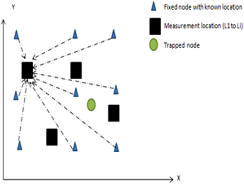
The trilateration algorithmic is a best-known traditional approach for localization of a node (Fig. 12.2). In the conventional trilateration algorithm, as shown in Fig. 12.2, there are three nodes, r1, r2 and r3, in fixed locations forming a triangle, with the middle node being the trapped node; using the Euclidian distance equation, the location of the trapped node can be estimated easily. Similarly, there is another approach to localization, namely location fingerprinting (Fig. 12.3). The location fingerprinting algorithm captures all RSSI values and represents those RSSI values on a logarithmic scale. The captured RSSI values are called a radio map and the array of the same is known as Radio Frequency (RF) signatures or fingerprinting. So, for the first location L1, the array is represented as

FIGURE 12.3 Location Fingerprinting Algorithm

s s L_{1} = [s s L_{l 1} s s L_{l 2} s s L_{l 3} \dots \dots \dots s s L_{l i}]

In this chapter, the sensor network will be designed in a well-known predefined disaster-prone path with the help of the technique of location fingerprinting. The RF signatures of all the vehicles moving all the way through the disaster-prone area are captured and will be communicated to the main central node. So, when the disaster happens, any vehicle can easily be tracked, using the appropriate RF signature.

12.3 Proposed Indigenous Sensor Network Ecosystem

Firstly, a network must be established in the disaster-prone area, using a fixed node, known as the anchor node, a visitor node (movable node) and a rescue operation node. The fixed node will be deployed in the predefined path and acts as a router node, which will direct the information from the visitor node location to the main central node. Visitor nodes are associated with visitors and act as coordinator nodes, which will continuously send the data to the anchor node (fixed node); the data refer to the RSSI. If the disaster happens, then the third node, known as the rescue operation node, will start the rescue process, acting as an end-device node. The fixed nodes are sufficiently intelligent to obtain the information from vehicles passing across it and making a radio map. As the vehicles are already registered at the registration point (see Fig. 12.4) far away from the disaster-prone area, updated information regarding the estimated location of vehicles, and also the number of vehicles, can be obtained at each and every point. Fig. 12.4 shows the block diagrams of the system and will show the roadmap of the disaster-prone area where the network is going to be deployed. The same information is routed through the fixed nodes to the registration point. So, a radio map can be designed at the registration point. As a result, in situations where disaster strikes, and fixed nodes become damaged, then the updated estimated location is safe at the registration points. The proposed system starts from the authentication point in the disaster-prone area i.e. Registration point 1 (Fig. 12.4), where the vehicle entry gets registered and the vehicle gets the wireless node. During the registration process, the number of persons and the vehicle number that is going to travel through that disaster-prone area will be noted down.

FIGURE 12.4 Basic setup of proposed Architecture

After the registration process in the wireless node, the vehicle enters the disaster-prone area and the wireless network is initialized. There are anchor nodes already present, which are communicating with the node present in the vehicle. The estimated location of the vehicle is updated all the time and data are logged wirelessly to the Registration point. As soon as the vehicle crosses the disaster-prone area endpoint, the smart device in the vehicle informs Registration point 2, and the data will be removed. This technique can make a radio map of the vehicle node. If a disaster happens, then the vehicle node will become the trapped node. The trapped node is now automatically localized with the rescue team node. The last-estimated location can be tracked by radio map and, after obtaining the estimated location, further localization will be done by the unilateral technique, using VPM (Vector Parameter-based Mapping) [25]. The overall setup of location fingerprinting can be better understood by reference to Fig. 12.5.

12.3.1 Proposed Technique and Algorithm

The aim of the algorithm is to reach the trapped node by the VPM (Vector Parameter-based Mapping) protocol. Firstly, the node will scout for the RSSI and thereby calculate the estimated distance. The RSSI results are stored in the local memory of the rescue team node. The node will calculate the least remote RSSI value and the information to search for the new location, to move toward the trapped node. The rescue team node continues its steps until it reaches the trapped node. The algorithm is independent of the other anchor nodes, unlike in the trilateration algorithm. In this section, we will first understand the VPM protocol and then the hybrid algorithm to achieve optimization of the designed algorithm.

12.3.2 VPM (Vector Parameter-based Mapping) Protocol

The VPM protocol is state-of-the-art design, based on the unilateral technique. The blue dot is the trapped node and the red dot is the node with the rescue or searching team (refer to Fig. 12.6). The disaster-prone area, where the node is trapped, is divided into the vectors. Let us surmise that the current location of the searching node is in position (x, y). Now the best possible move of the node is 90° in a direction toward (x′, y′) or (x″, y″). There is no situation where it can move to an angle greater than 90°, because this would lead to an increase in RSSI value. So, the maximal angle of movement will be 90°. If the searching node moves toward (x′, y′) or (x″, y″) to a distance x or moves toward (x‴, y‴) to a distance y, then it will obtain the same RSSI value, due to the omnidirectional behavior of the Xbee antenna. An important point to note is the distance $y ≺ x$ , so the node gets a stronger RSSI signal at (x‴, y‴) than at the points (x′, y′) or (x″, y″). So, the most tenable move of the searching node is toward (x‴, y‴), i.e., to an angle of 45°. Practically it will always be α° <90°. So, the new coordinates of the searching node will be (x‴, y‴). Again, the searching node maps the area through vectorization and moves accordingly toward the trapped node by an α° angle which is always less than (<) 90°. The rescue team node (pursuit node) always does the search training in +x, −x, +y and –y directions, and moves accordingly toward the anchor (target) node (refer to Fig. 12.7).

FIGURE 12.6 Approach toward Anchor Node-VPM Protocol-based Mapping

FIGURE 12.7 Training pattern in −X, X, −Y, Y direction, using VPM Protocol

The rescue team node (pursuit node) always does the search training in +x, −x, +y and –y directions, and moves accordingly toward the anchor (target) node (refer to Fig. 12.7).

12.3.3 Hybrid TLBO (Teaching–Learning-based Optimization) and Unilateral Technique

Localization of the node is carried out using two methods, i.e., LNSM (Log Normal Shadowing Method) and Hybrid TLBO-unilateral algorithm [25]. This hybrid algorithm is based on the classical approach of the TLBO algorithm [26] and a modified trilateration technique, i.e., unilateration, using the VPM protocol, which has already been explained in the previous section (Section 12.3.2).

In this section, RSSI values have been used for the localization process, as discussed in the literature survey. It has been observed during the experiments that the RSSI values fluctuate considerably or sometimes they fade too. To remove the problem of noisy channels, it is very important to model the wireless channel. For the LNSM approach, two nodes have been placed in outdoor locations. One of the nodes acted as an anchor (fixed) node and the other one as a pursuit node. Both nodes have been equipped with Xbee transceiver modules and are able to obtain the RSSI values. The RSSIs are captured in SD card module (in-built features of self-designed nodes). The pursuit node is put through to move around the anchor node and the estimated distance is calculated using LNSM, by obtaining the RSSI values. Using LNSM, the distance can easily be calculated, and localization of the nodes can be achieved. Once the nodes are modeled, then the localization technique is optimized further, using the hybrid TLBO-unilateral algorithm.

First, let us understand the classical approach of the TLBO. TLBO is a teacher–learner-based algorithm that mainly focuses on the learning given by the teacher node to the learner node, so that the best learner node will become the teacher node for other nodes. This will be explained further in detail later in this chapter and the unilateral algorithm is the improved version of the trilateration algorithm. So, in both experiments, RSSI values have been obtained and, through the RSSI values, the pursuit node is subject to discovering the trapped node.

12.3.3.1 Modeling of Wireless Channel

The propagation of the message signal via the wireless channel is very noisy, due to a number of environmental parameters. Therefore, it is recommended to model the channel before the transmission of RSSI values. To model the wireless channel, there are many proliferation models, like the free-space model, the two-ray model, LNSM (Log Normal Shadowing Model), etc. In this research, LNSM has been used because of its universal acceptance. LNSM is widely used in wireless sensor networks. The LNSM model has a feature to set the environmental parameters in real time. Hence, for any geographical as well as environmental situation, one can model the channel. The LNSM technique is discussed in detail in the next section (Section 12.3.3.2).

12.3.3.2 LNSM (Log-Normal Shadowing Model)

The RSSI signals from the wireless channel are very much prone to reflections, diffractions, and scattering. So, to tackle the problem of a noisy channel, it is important to model the wireless channels by analytical or empirical methods. In the research carried out here, the analytical method has been adopted for modeling the wireless channel. To model a wireless channel in this research, a node has been placed in the outside environment and strengthening of the signal has been observed till the pursuit and anchor nodes moved from 150 m to 1 m of distance apart. At a distance of 1 m, the signal strength should be −40 dBm in the case of ZigBee [27]. This is the first step to modeling the channel in the case of ZigBee.

To obtain the condition of the channel in an outdoor location, an experiment was conducted. Several trails have been made in aligning the pursuit node and anchor node. The pursuit node is made to move toward the anchor node from a different angle and direction. The maximum distance is kept at 150 m, although this distance can be increased. The outdoor location where the anchor node has been placed is almost flat. As already discussed, the nodes have been equipped with Xbee and SD card modules. For several trials, RSSI values have been captured and a dataset has been designed from where the estimated distance can be calculated [16]. It has been observed that

P_{L (d)} (d B m) = P_{L (d_{0})} + 10 n \log_{10} (\frac{d}{d_{0}}) + X_{σ}

(12.1)

where $P_{L (d)} (d B m)$ is the path loss at a distance d (meters), $P_{L (d_{0})}$ is the path loss at a distance d₀ (meters), d₀ is the reference distance, i.e., 1 meter as suggested for the Xbee module and, at 1 m, the strongest RSSI value, of −40 dBm. n is the path loss exponent calculated using the LNSM technique, and X _σ is the zero mean Gaussian random variable (in dB), with a standard deviation σ.

The RSSI values can be calculated as

RSSI = P_{t} (d B m) - P_{L (d)} (d B m)

(12.2)

where P _t(dBm) is the transmitted power from the node. So, the RSSI at the pursuit node will be

P_{L (d)} (d B m) = P_{L (d_{0})} + 10 n \log_{10} (\frac{d}{d_{0}}) + X_{σ}

(12.3)

The value of “n” (path loss exponent) can be calculated as shown in Table 12.1. The value of n will change for different geographical and environmental conditions

TABLE 12.1
Path Loss Exponent Values

S. No.	Path Loss Exponent (n)	Environment
1	2.0	Free space
2	1.6–1.8	Inside building (line of sight)
3	1.8	Supermarket Store
4	2.09	Conference room, with table and chairs
5	2.2	Factory
6	2–3	Inside factory (no line of sight)
7	2.8	Indoor residential area
8	2.4	Outdoor environment (this chapter)

12.3.3.3 Hybrid TLBO-Unilateral Algorithm

There is a need for optimization to minimize the distance error, using RSSI values to localize the trapped node. Here, the TLBO algorithm has been used for the optimization process. TLBO is a teacher–learner-based optimization algorithm. It is the best-suited algorithm as it indispensable for any algorithm-specific parameters, as with other algorithms. GA (Genetic Algorithm) is particularly dependent on some algorithm-specific parameters, like mutation probability or cross-over probability [28]; as with GA, the ABC (Artificial Bee colonial) algorithm [29] also needs some algorithm-specific parameters to configure, whereas PSO also requires its own parameters, like inertial weights, and social and cognitive parameters [30]. There are some other algorithms, such as ES (Evolution Strategy), DE (Differential Evolution), BBO (Biogeography-Based Optimizer), and AIA (Attack Intention Analysis), etc. that also requires some algorithm-specific parameters. The calibration of these parameters must be perfect, otherwise the convergence result will not be accurate and it will increase the computational efforts unnecessarily. The TLBO algorithm is one optimization technique in which one does not need to optimize such critical parameters. TLBO is divided into the teacher as well as the learner phase.

As discussed previously, the most classical approach to locating the trapped node is trilateration and a state-of-the-art unilateral technique has also been discussed to locate the trapped node. Particularly for this research, the unilateral algorithm is proposed, as it reduces the number of nodes in the network. Now, to optimize the localization process in terms of distance error, the hybrid TLBO-unilateral algorithm has been designed. In the hybrid algorithm, the pursuit node will forage for the RSSI and, once it receives the RSSI signal of the trapped node, it teaches the pursuit nodes to obtain the strongest RSSI value at that very first step. After the first step, the learner pursuit node will become the teacher pursuit node and starts searching for the strongest RSSI signal i.e. −40 dBm. The simulation of the designed algorithm is done in SCILAB. As discussed earlier, because of the outdoor location used for the experiments, the nodes have omnidirectional RF coverage. So, to solve the localization problem, the research developed a probability- based algorithm.

The equations below describe the localization method that combines the data obtained from the RSSI values with the actual position of the sensor. After the node gets trapped, let us assume that the estimated position of the trapped node is $P_{es_pos}$ and its exact position is $P_{ex_pos}$ . Probability theory states that

P_{d i} (P_{ex_pos}) = P (P_{es_pos} | P_{ex_pos})

(12.4)

In Eq. 12.4, the P _diis deployment probability field function for the anchor node. Consider the RSSI value, where the estimated probable distance is

P_{d i} (P_{ex_pos}) = \frac{1}{2 π σ_{x} σ_{y}} e^{[- (\frac{1}{2}) [\frac{{(x_{ex_pos} - x_{es_pos})}^{2}}{σ^{2}_{x}} + \frac{{(y_{ex_pos} - y_{es_pos})}^{2}}{σ^{2}_{y}}]]}

(12.5)

σ_{x} = x_{m} \cdot P, σ_{y} = y_{m} \cdot P

(12.6)

In Eq. 12.6, P is known as the error factor considered for the node. If the anchor node (ith node) receives the RSSI from the pursuit node (jth node), the distance between the two nodes can be estimated from RSSI values and the noisy estimated distance can be denoted as $d_{noise (i j)}$ . The probability function will be defined for the real position $P_{ex_pos_node_i}$ of the node with respect to the estimated node ${\hat{P}}_{es_pos_node_j}$

P_{(i, j)} (P_{d E_{i}}) = P (d_{noise(i j)} | P_{ex_pos_node_i}, {\hat{P}}_{es_pos_node_j})

(12.7)

Considering the noisy channel, the distance estimated is $d_{noise (i j)}$ . Now, as the RSSI values have a Gaussian distribution, so the probability function can be defined as

P (d_{noise(i j)} | P_{ex_pos_node_i}, {\hat{P}}_{es_pos_node_j}) = P (d_{noise(i j)} | \partial (P_{ex_pos_node_i}, {\hat{P}}_{es_pos_node_j}))

(12.8)

P (d_{noise(i j)} | P_{d E_{i}}, {\hat{P}}_{d E_{j}}) = \frac{1}{2 π d_{noise (i j)} r} e^{\frac{{(\partial (P_{ex_pos_node_i}, {\hat{P}}_{es_pos_node_j}) - d_{noise (i j)})}^{2}}{2 {(d_{noise (i j)} . r)}^{2}}}

(12.9)

In Eq. 12.9, r is the range error factor, which is considered to be 0.1 in our case.

Since the trapped node position and the RSSI measurement by the pursuit node are independent, the overall probability function can be combined by multiplication. Combining Eq. 12.7 and 12.9

\begin{matrix} F = \frac{{(x_{ex_pos} - x_{es_pos})}^{2}}{σ^{2}_{x}} + \frac{{(y_{ex_pos} - y_{es_pos})}^{2}}{σ^{2}_{y}} \\ + \sum_{j \in j_{i}}^{} \frac{{(\partial (P_{ex_pos_node_i}, {\hat{P}}_{es_pos_node_j}) - d_{noise(i j)})}^{2}}{2 {(d_{noise(i j)} . r)}^{2}} \end{matrix}

(12.10)

Eq. 12.10 is used to obtain the optimized distance error in a noisy channel.

12.4 Experimental Test Bed Set-Up in an Outdoor Location and the Design of Sensor Nodes

Wireless sensor node design is a significant component in managing a catastrophe, that will provide reliable communication under post-disaster conditions. The design of nodes, as reported in this section, is unique in this specified area of application, and no other solution has been found to be available in the literature, to the best of our knowledge. The node consists of a Xbee radio as a transceiver, and an SD card to describe the vital information of the adjacent nodes, especially the RSSI value, along with the time log, power bank, solar panel to charge the power bank, and an LCD display. In the present study, the nodes developed to manage the disaster are classified as: anchor node (fixed nodes), trapped node (visitor node), and a pursuit node (refer to Figs. 12.8 and 12.9). The hardware architecture of all the nodes is the same except for their role in the wireless network. The fixed nodes are routers which will route the location of the visitor node to the main central server, and each has the capability of an on-board data log mechanism. The trapped node (visitor) is the end-device node, which will interact with fixed nodes (routers) while it is moving in the disaster-prone area. If, in any case, the disaster happens, the trapped node can easily be localized by a pursuit node configured as the end-node. The detailed hardware/control architecture are shown in Fig. 12.8. Figs. 12.9 and 12.10 show the fixed nodes (anchor node), the visitor node (trapped node), and the pursuit node. The whole disaster-prone area is managed by the coordinator node. The coordinator node requests the information on a timely basis from the router nodes.

FIGURE 12.8 Detailed hardware/control architecture of Sensor Node

FIGURE 12.10 Visitor Node (Trapped Node) and Pursuit Node

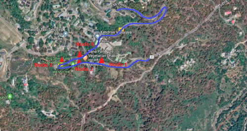
Many experiments have been conducted in outdoor locations with the designed nodes in the seismic zone of Himachal Pradesh (Dharamshala to McLeod Ganj) (Fig. 12.11). The experiments for this location have been conducted, keeping in mind the reliability of the network. In this section, the placement of nodes is discussed with respect to the coverage area. It is to be noted that, for a test-bed area of 150 m × 100 m, six nodes (four fixed, one pursuit, and one visitor node) are enough to perform the tests.

FIGURE 12.11 Node placement in OSA location (Dharamshala McLeod Ganj Road)

The exact positions of the fixed nodes have been estimated, keeping in mind the appropriate handshaking, whereas the visitor node is made to move from one fixed node to another fixed node. The visitor node can channelize and concede 20 bytes of data. The experiments on different test areas include the tests of RSSI (Received Signal Strength Indicator) w.r.t. the time.

12.5 Validation and Results of the Modified Approaches to Localization

12.5.1 Discussions on the Searching Pattern of Nodes

Fig. 12.12 shows the inquisitor pattern of the pursuit node, obtained using SCILAB. The virtual environment of SCILAB is designed for outdoor locations only. Fig. 12.12 presents the RSSI values in a test field. For a greater understanding, the figure is divided into upper and lower halves, which clearly show the path followed by the pursuit node to locate the trapped node. As mentioned in Fig. 12.12, as soon as the pursuit node receives the RSSI signal, it will also receive the nearby RSSI signals. In the simulation environment, the pursuit node gets the −117 dBm as its first RSSI signal, and the nearby signals presented are −109 dBm, −112 dBm, −121 dBm, −120 dBm, and −111 dBm. As per the VPM protocol, the pursuit node accepts the new location i.e. −109 dBm location, as 109 dBm is the strongest signal among them all. Now, according to the hybrid TLBO and the unilateral algorithm, the pursuit node learns from the teacher to move to the next location. By this technique, the teacher identifies the best learner. Similarly, the pursuit node moves ahead and gets the new location of –107 dBm, and the localization deed continues until the target node is located. This makes the anchor node fully discernible in any outside location. The advantage of this technique is its simplicity of getting embedded into most of the electronics embedded platform. The same is tested with respect to the hardware also and the trapped node is then fully discoverable in the outdoor environment.

FIGURE 12.12 Path as Computed by Hybrid TLBO-Unilateral Algorithm for outdoor location

12.5.2 Fingerprinting Technique Validation

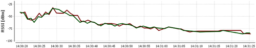
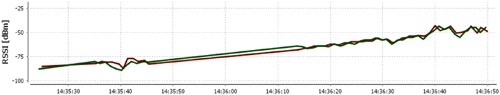
To validate the fingerprinting technique, a wireless network has been established in the disaster-prone area and experiments are conducted for validating the network, where RF signatures have been captured, and proper handshaking of the sensor node in the vehicle is searched for, with the fixed node deployed in the disaster-prone area. The methodology for the deployment of such a network has already been discussed in Section 12.3. As defined, the vehicles with their respective sensor nodes were made to move, and respective RF signatures were detected. The dereliction ratio of handshaking and capturing the RF signatures was much lower. The vehicle was made to pass the disaster-prone area at different speeds, i.e., from 20 km/h to 50 km/h. The packet loss was more when vehicle speed was more than 45 km/h and less when the vehicle speed was less than 40 km/h. The terrain was hilly, so the vehicle maximum speed was not more than 50 km/h. There is a loss of one or two packets only at speeds of more than 45 km/h. The results from handshaking of the nodes were also observed, when the vehicle is moving from location 1 to location 2, and to other location. The handshaking between the nodes was easy and smooth. RF values were captured in the fixed nodes. In Fig. 12.13, the RF signature was captured by fixed nodes of location 1, with the vehicle carrying the movable node. As captured, the signal varies from −90 dBm to −48 dBm. Similarly, when moving the MN1 away from the fixed node of location 1, then the signal was captured, and it varied from −40 dBm to −90 dBm, as shown in Fig. 12.14. The same scenario was observed for other locations too, as shown in location 2 and location 3 in Fig. 12.15 and Fig 12.16, respectively. In Fig. 12.17 it was observed that, if the speed of the vehicle exceeded 45 km/h, then packet loss took place. The packet loss is easily observed in Fig. 12.18. The results show the exceptional behavior of reliability of the fixed as well as the movable node.

FIGURE 12.13 RF signature by node in location 1 (vehicle carrying node moves toward fixed node in location 1)

FIGURE 12.14 RF signature by node in location 1 (vehicle carrying node moves away from fixed node in location 1)

FIGURE 12.15 RF signature by node in location 2 (vehicle carrying node moves away from node in location 2)

FIGURE 12.16 RF signature by node in location 3 (vehicle carrying node moves away from node in location 3)

FIGURE 12.17 RF signature by node in location 4 with speed of 48 km/h

FIGURE 12.18 RF signature by node in location 4 with speed of 25 km/h

12.6 Conclusion and Future Scopes

To achieve high-quality mobility in a disaster-prone area, sensor networks are one of the most promising technologies that automotive industries can adopt. This chapter discussed the design, development, and deployment of a sensor network for the mobility of vehicles in disaster-prone areas. The proposed sensor network has a capability of tracking trapped vehicles. The algorithms, such as location fingerprinting and unilateral techniques, were used to localize the vehicle, and these two algorithms are the backbone of the proposed network. The location fingerprinting technique is used to design the radio map by capturing the RF signatures used to track the vehicle in real time for pre-disaster as well as post-disaster situations. Many trails were conducted to validate the algorithm in simulation as well as in real time. The study was conducted over a limited area; in the future, we will extend the study to cover larger areas too and to cover other geographical areas. In future, we will also consider energy consumption in our study.

However, it must be noted that the developed system has not been designed for all disasters and for all geographical regions. This must be kept in mind with respect to the broad spectrum of the current study, thereby making it a larger task. However, should floods be considered the focal point of the node design, the details, especially its structure, will greatly change. In that case, it will be a completely different research study where one has to think of a floating node concept.

The proposed system improves the sustainability quotient, and also has a negligible impact on the environment. At the same time, its working is affected little by changes in the environmental conditions in the proposed areas. No harmful products are emitted into the environment. The system is not dependent on any infrastructure which might otherwise get destroyed in case of a disaster. The smaller occupied area also helps to maintain the ecological conservation of the geographical region. Even the maintenance and up-grading of the nodes, as well as the change in node locations, are not major tasks. The feature of reliable communication strongly favors sustainable development.

References

1. Brundtland, G. H. Our common future—Call for action. Environmental Conservation, 1987. 14(4): pp. 291–294.
2. Mukherjee, S., Analytical Modeling of Heterogeneous Cellular Networks. 2014. Cambridge University Press.
3. Usman, A. and S.H. Shami, Evolution of communication technologies for smart grid applications. Renewable and Sustainable Energy Reviews, 2013. 19: pp. 191–199.
4. Berke, P.R., J. Kartez, and D. Wenger, Recovery after disaster: achieving sustainable development, mitigation and equity. Disasters, 1993. 17(2): pp. 93–109.
5. Pearce, L., Disaster management and community planning, and public participation: how to achieve sustainable hazard mitigation. Natural Hazards, 2003. 28(2–3): pp. 211–228.
6. O’Brien, G., et al., Climate change and disaster management. Disasters, 2006. 30(1): pp. 64–80.
7. Bello, O.M. and Y.A. Aina, Satellite remote sensing as a tool in disaster management and sustainable development: towards a synergistic approach. Procedia-Social and Behavioral Sciences, 2014. 120: pp. 365–373.
8. Shaw, R., F. Mallick, and A. Islam, Disaster Risk Reduction Approaches in Bangladesh. 2013. Springer.
9. Sahay, B., N.V.C. Menon, and S. Gupta, Humanitarian logistics and disaster management: the role of different stakeholders, in Managing Humanitarian Logistics. 2016, Springer. pp. 3–21.
10. Ooi, G.L., et al., Near real-time landslide monitoring with the smart soil particles. Japanese Geotechnical Society Special Publication, 2016. 2(28): pp. 1031–1034.
11. Gioia, E., et al., Application of a process-based shallow landslide hazard model over a broad area in Central Italy. Landslides, 2016. 13(5): pp. 1197–1214.
12. Wu, C.-I., et al., An intelligent slope disaster prediction and monitoring system based on WSN and ANP. Expert Systems with Applications, 2014. 41(10): pp. 4554–4562.
13. Kohvakka, M., et al. Performance analysis of IEEE 802.15. 4 and ZigBee for large-scale wireless sensor network applications. in Proceedings of the 3rd ACM International Workshop on Performance Evaluation of Wireless ad hoc, Sensor and Ubiquitous Networks. 2006. ACM.
14. Ali, A., et al., Efficient predictive monitoring of wireless sensor networks. International Journal of Autonomous and Adaptive Communications Systems, 2012. 5(3): pp. 233–254.
15. Hartenstein, H. and L. Laberteaux, A tutorial survey on vehicular ad hoc networks. IEEE Communications Magazine, 2008. 46(6): 164–171.
16. Gharghan, S.K., et al., Accurate wireless sensor localization technique based on hybrid PSO-ANN algorithm for indoor and outdoor track cycling. IEEE Sensors Journal, 2016. 16(2): pp. 529–541.
17. Nedjati, A., B. Vizvari, and G. Izbirak, Post-earthquake response by small UAV helicopters. Natural Hazards, 2016. 80(3): pp. 1669–1688.
18. Zhou, Y., et al., Multi-UAV-aided networks: aerial-ground cooperative vehicular networking architecture. Ieee Vehicular Technology Magazine, 2015. 10(4): pp. 36–44.
19. Tuna, G., B. Nefzi, and G. Conte, Unmanned aerial vehicle-aided communications system for disaster recovery. Journal of Network and Computer Applications, 2014. 41: pp. 27–36.
20. Rusu, C.V. and H.-S. Ahn . Optimal network localization by particle swarm optimization. in Intelligent Control (ISIC), 2011 IEEE International Symposium on. 2011. IEEE.
21. Payal, A., C.S. Rai, and B.R. Reddy, Analysis of some feedforward artificial neural network training algorithms for developing localization framework in wireless sensor networks. Wireless Personal Communications, 2015. 82(4): pp. 2519–2536.
22. Thongpul, K., N. Jindapetch, and W. Teerapakajorndet . A neural network based optimization for wireless sensor node position estimation in industrial environments. in Electrical Engineering/Electronics Computer Telecommunications and Information Technology (ECTI-CON), 2010 International Conference on. 2010. IEEE.
23. Nerguizian, C. and V. Nerguizian . Indoor fingerprinting geolocation using wavelet-based features extracted from the channel impulse response in conjunction with an artificial neural network. in Industrial Electronics, 2007. ISIE 2007. IEEE International Symposium on. 2007. IEEE.
24. Rahman, M.S., Y. Park, and K.-D. Kim, RSS-based indoor localization algorithm for wireless sensor network using generalized regression neural network. Arabian Journal for Science and Engineering, 2012. 37(4): pp. 1043–1053.
25. Kaundal, V., P. Sharma, and M. Prateek, Wireless sensor node localization based on LNSM and hybrid TLBO-unilateral technique for outdoor location. International Journal of Electronics and Telecommunications, 2017. 63(4): pp. 389–397.
26. Rao, R.V., Teaching-learning-based optimization algorithm, in Teaching Learning Based Optimization Algorithm. 2016, Springer. pp. 9–39.
27. ZigBee Specification, ZigBee Alliance. ZigBee Document 053474r06, Version, 2006. 1.
28. Elsayed, S.M., R.A. Sarker, and D.L. Essam, A new genetic algorithm for solving optimization problems. Engineering Applications of Artificial Intelligence, 2014. 27: pp. 57–69.
29. Karaboga, D., et al., A comprehensive survey: artificial bee colony (ABC) algorithm and applications. Artificial Intelligence Review, 2014. 42(1): pp. 21–57.
30. Cao, C., Q. Ni, and X. Yin, Comparison of particle swarm optimization algorithms in wireless sensor network node localization. in Systems, Man and Cybernetics (SMC), 2014 IEEE International Conference on. 2014. IEEE. pp. 252–257.

Table of Contents for Chapter 12 Developing Ecosystem for Tracking Vehicles in Disaster Prone Areas

Create new playlist

Sign In

Sign Up

Table of Contents for
Chapter 12 Developing Ecosystem for Tracking Vehicles in Disaster Prone Areas