Chapter 5. Dealing With Few to No Labels
There is one question so deeply ingrained into every data scientist’s mind that it’s usually the first thing they ask at the start of a new project: is there any labeled data? More often than not, the answer is “no” or “a little bit”, followed by an expectation from the client that your team’s fancy machine learning models should still perform well. Since training models on very small datasets does not typically yield good results, one obvious solution is to annotate more data. However, this takes time and can be very expensive, especially if each annotation requires domain expertise to validate.
Fortunately, there are several methods that are well suited for dealing with few to no labels! You may already be familiar with some of them such as zero-shot or few-shot learning from GPT-3’s impressive ability to perform a diverse range of tasks from just a few dozen examples.
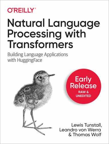
In general, the best performing method will depend on the task, the amount of available data and what fraction is labeled. A decision tree is shown in Figure 5-1 to help guide us through the process.
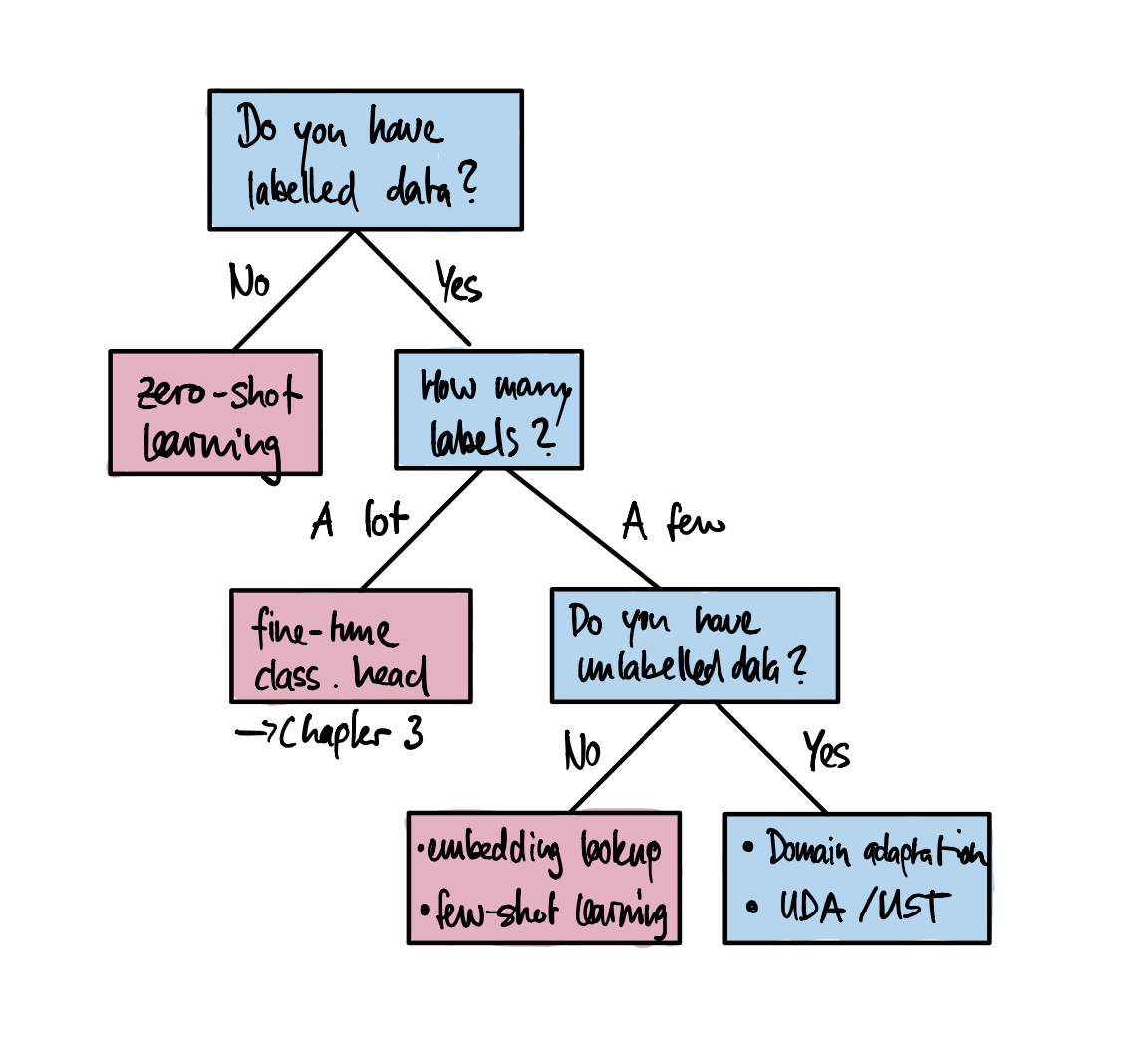
Figure 5-1. Several techniques that can be used to improve model performance in the absence of large amounts of labeled data.
Let’s walk through this decision tree step-by-step:
- Do you have labelled data?
-
Even a handful of labeled samples can make a difference as to which method works best. If you have no labeled data at all, you can start with the zero-shot learning approach in SECTION X, which often sets a strong baseline to work from.
- How many labels?
-
If labeled data is available, the deciding factor is how much? If you have a lot of training data available you can use the standard fine-tuning approach discussed in Chapter 1.
- Do you have unlabeled data?
-
If you only have a handful of labeled samples it can immensely help if you have access to large amounts of unlabeled data. If you have access to unlabeled data you can either use it to fine-tune the language model on the domain before training a classifier or you can use more sophisticated methods such as Universal Data Augmentation (UDA)1 or Uncertainty-Aware Self-Training (UST)2. If you also don’t have any unlabeled data available it means that you cannot even annotate more data if you wanted to. In this case you can use few-shot learning or use the embeddings from a pretrained language model to perform look-ups with a nearest neighbor search.
In this chapter we’ll work our way through this decision tree by tackling a common problem facing many support teams that use issue trackers like Jira or GitHub to assist their users: tagging issues with metadata based on the issue’s description. These tags might define the issue type, the product causing the problem, or which team is responsible for handling the reported issue. Automating this process can have a big impact on productivity and enables the support teams to focus on helping their users. As a running example, we’ll use the GitHub issues associated with a popular open-source project: Hugging Face Transformers! Let’s now take a look at what information is contained in these issues, how to frame the task, and how to get the data.
Note
The methods presented in this chapter work well for text classification, but other techniques such as data augmentation may be necessary for tackling more complex tasks like named entity recognition, question answering or summarization.
Building a GitHub Issues Tagger
If you navigate to the Issues tab of the Transformers repository, you’ll find issues like the one shown in Figure 5-2, which contains a title, description, and a set of tags or labels that characterize the issue. This suggests a natural way to frame the supervised learning task: given a title and description of an issue, predict one or more labels. Since each issue can be assigned a variable number of labels, this means we are dealing with a multilabel text classification problem. This problem is usually more challenging than the multiclass setting that we encountered in Chapter 1, where each tweet was assigned to only one emotion.
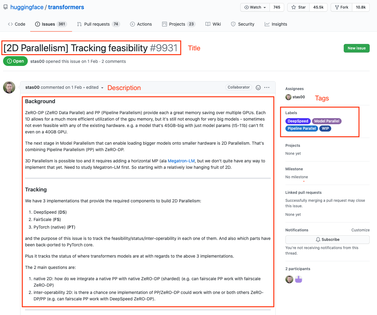
Figure 5-2. An typical GitHub issue on the Transformers repository.
Now that we’ve seen what the GitHub issues look like, let’s look at how we can download them to create our dataset.
Getting the Data
To grab all the repository’s issues we’ll use
the GitHub REST API to poll the
Issues
endpoint. This endpoint returns a list of JSON objects, where each
element contains a large number of fields about the issue including its
state (open or closed), who opened the issue, as well as the title,
body, and labels we saw in Figure 5-2. To poll the
endpoint, you can run the following curl command to download the first
issue on the first page:
curl "https://api.github.com/repos/huggingface/transformers/issues?page=1&per_page=1"
Since it takes a while to fetch all the issues, we’ve
included an issues.jsonl file in this book’s GitHub
repository, along with a fetch_issues function to
download them yourself.
Note
The GitHub REST API treats pull requests as issues, so our dataset contains a mix of both. To keep things simple, we’ll develop our classifier for both types of issue, although in practice you might consider building two separate classifiers to have more fine-grained control over the model’s performance.
Preparing the Data
Once we’ve downloaded all the issues, we can load them using Pandas:
importpandasaspddf_issues=pd.read_json("data/chapter07/issues.jsonl",lines=True)(f"DataFrame shape: {df_issues.shape}")
DataFrame shape: (9930, 26)
There are almost 10,000 issues in our dataset and by looking at a single row we can see that the retrieved information from the GitHub API contains many fields such as URLs, IDs, dates, users, title, body, as well as labels:
cols=["url","id","title","user","labels","state","created_at","body"]df_issues.loc[2,cols].to_frame()
| 2 | |
|---|---|
| url | https://api.github.com/repos/huggingface/trans... |
| id | 849529761 |
| title | [DeepSpeed] ZeRO stage 3 integration: getting ... |
| user | {'login’: ’stas00', ‘id’: 10676103, ‘node_id’:... |
| labels | [{'id’: 2659267025, ‘node_id’: ‘MDU6TGFiZWwyNj... |
| state | open |
| created_at | 2021-04-02 23:40:42 |
| body | **[This is not yet alive, preparing for the re... |
The labels columns is the thing that we’re interested in,
and each row contains a list of JSON objects with metadata about each
label:
[{"id":2659267025,"node_id":"MDU6TGFiZWwyNjU5MjY3MDI1","url":"https://api.github.com/repos/huggingface/transformers/labels/DeepSpeed","name":"DeepSpeed","color":"4D34F7","default":false,"description":""}]
For our purposes, we’re only interested in the name field
of each label object, so let’s overwrite the labels column
with just the label names:
df_issues["labels"]=(df_issues["labels"].apply(lambdax:[meta["name"]formetainx]))df_issues["labels"].head()
0             []
1             []
2    [DeepSpeed]
3             []
4             []
Name: labels, dtype: object
df_issues["labels"].apply(lambdax:len(x)).value_counts()
0    6440
1    3057
2     305
3     100
4      25
5       3
Name: labels, dtype: int64
Next let’s take a look at the top-10 most frequent labels in
the dataset. In Pandas we can do this by “exploding” the labels
column so that each label in the list becomes a row, and then we simply
count the occurrence of each label:
df_counts=df_issues["labels"].explode().value_counts()(f"Number of labels: {len(df_counts)}")df_counts.head(10)
Number of labels: 65
wontfix               2284
model card             649
Core: Tokenization     106
New model               98
Core: Modeling          64
Help wanted             52
Good First Issue        50
Usage                   46
Core: Pipeline          42
TensorFlow              41
Name: labels, dtype: int64
We can see that there are 65 unique labels in the dataset and that the
classes are very imbalanced, with wontfix and model card being the
most common labels. To make the classification problem more tractable,
we’ll focus on building a tagger for a subset of the labels.
For example, some labels such as Good First Issue or Help Wanted are
potentially very difficult to predict from the issue’s
description, while others such as the model card could be classified
with a simple rule that detects when a model card is added on the
Hugging Face Hub.
The following code shows the subset of labels that we’ll work with, along with a standardization of the names to make them easier to read:
label_map={"Core: Tokenization":"tokenization","New model":"new model","Core: Modeling":"model training","Usage":"usage","Core: Pipeline":"pipeline","TensorFlow":"tensorflow or tf","PyTorch":"pytorch","Examples":"examples","Documentation":"documentation"}deffilter_labels(x):return[label_map[label]forlabelinxiflabelinlabel_map]df_issues["labels"]=df_issues["labels"].apply(filter_labels)all_labels=list(label_map.values())
Now let’s look at the distribution of the new labels:
df_counts=df_issues["labels"].explode().value_counts()df_counts
tokenization        106
new model            98
model training       64
usage                46
pipeline             42
tensorflow or tf     41
pytorch              37
documentation        28
examples             24
Name: labels, dtype: int64
Since multiple labels can be assigned to a single issue we can also look at the distribution of label counts:
df_issues["labels"].apply(lambdax:len(x)).value_counts()
0    9489
1     401
2      35
3       5
Name: labels, dtype: int64
The vast majority of the issues have no labels at all, and only a handful have more than one. Later in this chapter we’ll find it useful to treat the unlabeled issues as a separate training split, so let’s create a new column that indicates whether the issues is unlabeled or not:
df_issues["split"]="unlabelled"mask=df_issues["labels"].apply(lambdax:len(x))>0df_issues.loc[mask,"split"]="labelled"df_issues["split"].value_counts()
unlabelled    9489
labelled       441
Name: split, dtype: int64
Let’s now take a look at an example:
forcolumnin["title","body","labels"]:(f"{column}: {df_issues[column].iloc[26][:200]}")
title: Add new CANINE model

body: # New model addition

## Model description

Google recently proposed a new **C**haracter **A**rchitecture with **N**o
 > tokenization **I**n **N**eural **E**ncoders architecture (CANINE). Not only

labels: ['new model']
In this example a new model architecture is proposed, so the new model
tag makes sense. We can also see that the title contains information
that will be useful for our classifier, so let’s concatenate
it with the issue’s description in the body field:
df_issues["text"]=(df_issues.apply(lambdax:x["title"]+""+x["body"],axis=1))
As we’ve done in other chapters, it a good idea to have a quick look at the number of words in our texts to see if we’ll lose much information during the tokenization step:
importnumpyasnp(df_issues["text"].str.split().apply(len).hist(bins=np.linspace(0,5000,101),grid=False));

The distribution has a characteristic long tail of many text datasets. Most texts are fairly short but there are also issues with more than 1,000 words. It is common to have very long issues especially when error messages and code snippets are posted along with it.
Creating Training Sets
Now that we’ve explored and cleaned our dataset, the final thing to do is define our training sets to benchmark our classifiers.
We want to make sure that splits are balanced which is a bit trickier
for a multlilabel problem because there is no guaranteed balance for all
labels. However, it can be approximated an although scikit-learn does
not support this we can use the scitkit-multilearn
library which is setup for multilabel problems. The first thing we need
to do is transform our set of labels like pytorch and tokenization
into a format that the model can process. Here we can use
Scikit-Learn’s MultiLabelBinarizer transformer class,
which takes a list of label names and creates a vector with zeros for
absent labels and ones for present labels. We can test this by fitting
MultiLabelBinarizer on all_labels to learn the mapping from label
name to ID as follows:
fromsklearn.preprocessingimportMultiLabelBinarizermlb=MultiLabelBinarizer()mlb.fit([all_labels])mlb.transform([['tokenization','new model'],['pytorch']])
array([[0, 0, 0, 1, 0, 0, 0, 1, 0],
       [0, 0, 0, 0, 0, 1, 0, 0, 0]])
In this simple example we can see the first row has two ones
corresponding to the tokenization and new model labels, while the
second row has just one hit with pytorch.
To create the splits we can use the iterative_train_test_split
function which creates the train/test splits iteratively to achieve
balanced labels. We wrap it in a function that we can apply to
DataFrames. Since the function expects a two-dimensional feature
matrix we need to add a dimension to the possible indices before making
the split:
fromskmultilearn.model_selectionimportiterative_train_test_splitdefbalanced_split(df,test_size=0.5):ind=np.expand_dims(np.arange(len(df)),axis=1)labels=mlb.transform(df["labels"])ind_train,_,ind_test,_=iterative_train_test_split(ind,labels,test_size)returndf.iloc[ind_train[:,0]],df.iloc[ind_test[:,0]]
With that function in place we can split the data into supervised and unsupervised datasets and create balanced train, validation, and test sets for the supervised part:
fromsklearn.model_selectionimporttrain_test_splitdf_clean=df_issues[["text","labels","split"]].reset_index(drop=True).copy()df_unsup=df_clean.loc[df_clean["split"]=="unlabelled",["text","labels"]]df_sup=df_clean.loc[df_clean["split"]=="labelled",["text","labels"]]np.random.seed(0)df_train,df_tmp=balanced_split(df_sup,test_size=0.5)df_valid,df_test=balanced_split(df_tmp,test_size=0.5)
Finally, let’s create a DatasetDict with all the splits so
that we can easily tokenize the dataset and integrate with the
Trainer. Here we’ll use the nifty Dataset.from_pandas
function from Datasets to load each split directly from the
corresponding Pandas DataFrame:
fromdatasetsimportDataset,DatasetDictds=DatasetDict({"train":Dataset.from_pandas(df_train.reset_index(drop=True)),"valid":Dataset.from_pandas(df_valid.reset_index(drop=True)),"test":Dataset.from_pandas(df_test.reset_index(drop=True)),"unsup":Dataset.from_pandas(df_unsup.reset_index(drop=True))})ds
DatasetDict({
    train: Dataset({
        features: ['text', 'labels'],
        num_rows: 223
    })
    valid: Dataset({
        features: ['text', 'labels'],
        num_rows: 108
    })
    test: Dataset({
        features: ['text', 'labels'],
        num_rows: 110
    })
    unsup: Dataset({
        features: ['text', 'labels'],
        num_rows: 9489
    })
})
This looks good, so the last thing to do is to create some training slices so that we can evaluate the performance of each classifier as a function of the training set size.
Creating Training Slices
The dataset has the two characteristics that we’d like to
investigate in this chapter: sparse labeled data and mutlilabel
classification. The training set consists of only 220 examples to train
with which is certainly a challenge even with transfer learning. To
drill-down into how each method in this chapter performs with little
labelled data, we’ll also create slices of the training data
with even fewer samples. We can then plot the number of samples against
the performance and investigate various regimes. We’ll start
with only 8 samples per label and build up until the slice covers the
full training set using the iterative_train_test_split function:
np.random.seed(0)all_indices=np.expand_dims(list(range(len(ds["train"]))),axis=1)indices_pool=all_indiceslabels=mlb.transform(ds["train"]["labels"])train_samples=[8,16,32,64,128]train_slices,last_k=[],0fori,kinenumerate(train_samples):# split off samples necessary to fill the gap to the next split sizeindices_pool,labels,new_slice,_=iterative_train_test_split(indices_pool,labels,(k-last_k)/len(labels))last_k=kifi==0:train_slices.append(new_slice)else:train_slices.append(np.concatenate((train_slices[-1],new_slice)))# add full dataset as last slicetrain_slices.append(all_indices),train_samples.append(len(ds["train"]))train_slices=[np.squeeze(train_slice)fortrain_sliceintrain_slices]
Great, we’ve finally prepared our dataset into training splits - let’s next take a look at training a strong baseline model!
Implementing a Bayesline
Whenever you start a new NLP project, it’s always a good idea to implement a set of strong baselines for two main reasons:
-
A baseline based on regular expressions, hand-crafted rules, or a very simple model might already work really well to solve the problem. In these cases, there is no reason to bring out big guns like transformers which are generally more complex to deploy and maintain in production environments.
-
The baselines provide sanity checks as you explore more complex models. For example, suppose you train BERT-large and get an accuracy of 80% on your validation set. You might write it off as a hard dataset and call it a day. But what if you knew that a simple classifier like logistic regression gets 95% accuracy? That would raise your suspicion and prompt you to debug your model.
So let’s start our analysis by training a baseline model.
For text classification, a great baseline is a Naive Bayes classifier
as it is very simple, quick to train, and fairly robust to perturbations
in the inputs. The Scikit-Learn implementation of Naive Bayes does not
support multilabel classification out-of-the-box, but fortunately we can
again use the scitkit-multilearn library to cast the problem as a
one-vs-rest classification task where we train label_ids column in our training
sets. Here we can use the Dataset.map function to take care of all the
processing in one go:
defprepare_labels(batch):batch['label_ids']=mlb.transform(batch['labels'])returnbatchds=ds.map(prepare_labels,batched=True)
To measure the performance of our classifiers, we’ll use the
micro and macro defaultdict with a list to store the scores per split:
fromcollectionsimportdefaultdictmacro_scores,micro_scores=defaultdict(list),defaultdict(list)
Now we’re finally ready to train our baseline! Here’s the code to train the model and evaluate our classifier across increasing training set sizes:
fromsklearn.naive_bayesimportMultinomialNBfromsklearn.metricsimportclassification_reportfromskmultilearn.problem_transformimportBinaryRelevancefromsklearn.feature_extraction.textimportCountVectorizerfortrain_sliceintrain_slices:# Get training slice and test datads_train_sample=ds["train"].select(train_slice)y_train=np.array(ds_train_sample["label_ids"])y_test=np.array(ds["test"]["label_ids"])# Use a simple count vectorizer to encode our texts as token countscount_vect=CountVectorizer()X_train_counts=count_vect.fit_transform(ds_train_sample["text"])X_test_counts=count_vect.transform(ds["test"]["text"])# Create and train our model!classifier=BinaryRelevance(classifier=MultinomialNB())classifier.fit(X_train_counts,y_train)# Generate predictions and evaluatey_pred_test=classifier.predict(X_test_counts)clf_report=classification_report(y_test,y_pred_test,target_names=mlb.classes_,zero_division=0,output_dict=True)# Store metricsmacro_scores["Naive Bayes"].append(clf_report["macro avg"]["f1-score"])micro_scores["Naive Bayes"].append(clf_report["micro avg"]["f1-score"])
There’s quite a lot going on in this block of code, so
let’s unpack it. First, we get the training slice and encode
the labels. Then we use a count vectorizer to encode the texts by simply
creating a vector of the size of the vocabulary where each entry
corresponds to the frequency a token appeared in the text. This is
called a bag-of-word approach since all information on the order of the
words is lost. Then we train the classifier and use the prediction on
the test set to get the micro and macro
With the following helper function we can plot the results of this experiment:
importmatplotlib.pyplotaspltdefplot_metrics(micro_scores,macro_scores,sample_sizes,current_model):fig,(ax0,ax1)=plt.subplots(1,2,figsize=(10,5),sharey=True)forruninmicro_scores.keys():ifrun==current_model:ax0.plot(sample_sizes,micro_scores[run],label=run,linewidth=2)ax1.plot(sample_sizes,macro_scores[run],label=run,linewidth=2)else:ax0.plot(sample_sizes,micro_scores[run],label=run,linestyle="dashed")ax1.plot(sample_sizes,macro_scores[run],label=run,linestyle="dashed")ax0.set_title("Micro F1 scores")ax1.set_title("Macro F1 scores")ax0.set_ylabel("Test set F1 score")foraxin[ax0,ax1]:ax.set_xlabel("Number of training samples")ax.legend(loc="upper left")ax.set_xscale("log")ax.set_xticks(sample_sizes)ax.set_xticklabels(sample_sizes)ax.minorticks_off()plt.tight_layout()plot_metrics(micro_scores,macro_scores,train_samples,"Naive Bayes")

Note that we plot the number of samples on a logarithmic scale. From the
figure we can see that the performance on the micro and macro
Working With No Labeled Data
The first technique that we’ll consider is zero-shot classification, which is suitable in settings where you have no labeled data at all. This setting is suprisingly common in industry, and might occur because there is no historic data with labels or acquiring the labels for the data is difficult to get. We will cheat a bit in this section since we will still use the test data to measure the performance but we will not use any data to train the model. Otherwise the comparison to the following approaches would be difficult. Let’s now look at how zero-shot classification works.
Zero-Shot Classification
The goal of zero-shot classification is to make use of a pretrained model without any additional fine-tuning on your task-specific corpus. To get a better idea of how this could work, recall that language models like BERT are pretrained to predict masked tokens in text from thousands of books and large Wikipedia dumps. To successfully predict a missing token the model needs to be aware of the topic in the context. We can try to trick the model into classifying a document for us by providing a sentence like:
“This section was about the topic [MASK].”
The model should then give a reasonable suggestion for the document’s topic since this is a natural text to occur in the dataset.3
Let’s illustrate this further with the following toy
problem: suppose you have two children and one of them likes movies with
cars while the other enjoys movies with animals better. Unfortunately,
they have already seen all the ones you know so you want to build
function that tells you what topic a new movie is about. Naturally you
turn to transformers for this task, so the first thing to try loading
BERT-base in the fill-mask pipeline which uses the masked language
model to predict the content of the masked tokens:
fromtransformersimportpipelinepipe=pipeline("fill-mask",model="bert-base-uncased")
Next, let’s construct a little movie description and add a
prompt to it with a masked word. The goal of the prompt is to guide the
model to help us make a classification. The fill-mask pipeline returns
the most likely tokens to fill in the masked spot:
movie_desc="The main characters of the movie madacascarare a lion, a zebra, a giraffe, and a hippo. "prompt="The movie is about [MASK]."output=pipe(movie_desc+prompt)forelementinoutput:(f"class {element['token_str']}:{element['score']:.3f}%")
class animals:  0.103%
class lions:    0.066%
class birds:    0.025%
class love:     0.015%
class hunting:  0.013%
Clearly, the model predicts only tokens that are related to animals. We can also turn this around and instead of getting the most likely tokens we can query the pipeline for the probability of a few given tokens. For this task we might choose cars and animals so we can pass them to the pipeline as targets:
output=pipe(movie_desc+prompt,targets=["animals","cars"])forelementinoutput:(f"class {element['token_str']}:{element['score']:.3f}%")
class animals:  0.103%
class cars:     0.001%
Unsurprisingly, the probability for the token cars is much smaller than for animals. Let’s see if this also works for a description that is closer to cars:
movie_desc="In the movie transformers alienscan morph into a wide range of vehicles."output=pipe(movie_desc+prompt,targets=["animals","cars"])forelementinoutput:(f"class {element['token_str']}:{element['score']:.3f}%")
class cars:     0.139%
class animals:  0.006%
It worked! This is only a simple example and if we want to make sure it works well we should test it thoroughly but it illustrates the key idea of many approaches discussed in this chapter: find a way to adapt a pretrained model for another task without training it. In this case we setup a prompt with a mask in a way that we can use a masked language model directly for classification. Let’s see if we can do better by adapting a model that has been fine-tuned on a task that’s closer to text classification: natural language inference or NLI for short.
Hijacking Natural Language Inference
Using the masked language model for classification is a nice trick but we can do better still by using a model that has been trained on a task that is closer to classification. There is a neat proxy task called text entailment that can be used to train models for just this task. In text entailment, the model needs to determine whether two text passages are likely to follow or contradict each other. With datasets such as the Multi-Genre NLI Corpus (MNLI)4 or its multilingual counterpart the Cross-Lingual NLI Corpus (XNLI)5 a model is trained to detect entailments and contraditions.
Each sample in these dataset is composed of three parts: a premise, a hypothesis, and a label where the label can be one of “entailment”, “neutral”, and “contradiction”. The “entailment” label is given when the hypothesis text is necessarily true under the premise. The “contradiction” label is used when the hypothesis is necessarily false or inappropriate under the premise. If neither of these cases applies then the “neutral” label is assigned. See the figure Figure 5-3 for examples of the dataset.
Figure 5-3. Three examples from the MNLI dataset from three different domains. Image from MNLI paper.
Now it turns our that we can hijack a model trained on the MNLI dataset to build a classifier without needing any labels at all! The key idea is to treat the text we wish to classify as the premise, and then formulate the hypothesis as
“This example is about {label}.”
where we insert the class name for the label. The entailment score then tells us how likely that premise is about that topic, and we can run this for any number of classes sequentially. The downside of this is that we need to execute a forward pass for each class which makes it less efficient than a standard classifier. Another slightly tricky aspect is that the choice of label names can have a large impact on the accuracy, and choosing labels with semantic meaning is generally the best approach. For example if a label is simply called “Class 1”, the model has no hint what this might mean and whether this constitutes a contradiction or entailment.
The Transformers library has an MNLI model for zero-shot classification
built in. We can initialize it via the pipeline API as follows:
fromtransformersimportpipelinepipe=pipeline("zero-shot-classification",device=0)
The setting device=0 makes sure that the model runs on the GPU instead
of the default CPU to speed up inference. To classify a text we simply
need to pass it to the pipeline along with the label names. In addition
we can set multi_label=True to ensure that all the scores are returned
and not only the maximum for single label classification:
sample=ds["train"][0]("label:",sample["labels"])output=pipe(sample["text"],all_labels,multi_label=True)(output["sequence"])("predictions:")forlabel,scoreinzip(output["labels"],output["scores"]):(f"{label}, {score:.2f}")
label: ['new model'] Add new CANINE model # New model addition ## Model description Google recently proposed a new **C**haracter **A**rchitecture with **N**o > tokenization **I**n **N**eural **E**ncoders architecture (CANINE). Not only > the title is exciting: > Pipelined NLP systems have largely been superseded by end-to-end neural > modeling, yet nearly all commonly-used models still require an explicit > tokenization step. While recent tokenization approaches based on data-derived > subword lexicons are less brittle than manually engineered tokenizers, these > techniques are not equally suited to all languages, and the use of any fixed > vocabulary may limit a model's ability to adapt. In this paper, we present > CANINE, a neural encoder that operates directly on character sequences, > without explicit tokenization or vocabulary, and a pre-training strategy that > operates either directly on characters or optionally uses subwords as a soft > inductive bias. To use its finer-grained input effectively and efficiently, > CANINE combines downsampling, which reduces the input sequence length, with a > deep transformer stack, which encodes context. CANINE outperforms a > comparable mBERT model by 2.8 F1 on TyDi QA, a challenging multilingual > benchmark, despite having 28% fewer model parameters. Overview of the architecture:  Paper is available [here](https://arxiv.org/abs/2103.06874). We heavily need this architecture in Transformers (RIP subword tokenization)! The first author (Jonathan Clark) said on > [Twitter](https://twitter.com/JonClarkSeattle/status/1377505048029134856) > that the model and code will be released in April :partying_face: ## Open source status * [ ] the model implementation is available: soon > [here](https://caninemodel.page.link/code) * [ ] the model weights are available: soon > [here](https://caninemodel.page.link/code) * [x] who are the authors: @jhclark-google (not sure), @dhgarrette, @jwieting > (not sure) predictions: new model, 0.98 tensorflow or tf, 0.37 examples, 0.34 usage, 0.30 pytorch, 0.25 documentation, 0.25 model training, 0.24 tokenization, 0.17 pipeline, 0.16
Note
Since we are using a subword tokenizer we can even pass code to the model! Since the pretraining dataset for the zero-shot pipeline likely contains just a small fraction of code snippets, the tokenization might not be very efficient but since the code is also made up of a lot of natural words this is not a big issue. Also, the code block might contain important information such as the framework (PyTorch or TensorFlow).
We can see that the model is very confident that this text is about tokenization but it also produces relatively high scores for the other labels. An important aspect for zero-shot classification is the domain we operate in. The texts we are dealing with which are very technical and mostly about coding, which makes them quite different from the original text distribution in the MNLI dataset. Thus it is not surprising that this is a very challenging task for the model. For some domains the model might work much better than others, depending on how close they are to the training data.
Let’s write a function that feeds a single example through
the zero-shot pipeline, and then scale it out to the whole validation
set by running Dataset.map:
defzero_shot_pipeline(example):output=pipe(example["text"],all_labels,multi_label=True)example["predicted_labels"]=output["labels"]example["scores"]=output["scores"]returnexampleds_zero_shot=ds["valid"].map(zero_shot_pipeline)
Now that we have our scores, the next step is to determines which set of labels should be assigned to each example. Here there are a few options we can experiment with:
-
Define a threshold and select all labels above the threshold.
-
Pick the top-
To help us with determine which method is best, let’s write
a get_preds function that applies one of the methods to retrieve the
predictions:
defget_preds(example,threshold=None,topk=None):preds=[]ifthreshold:forlabel,scoreinzip(example["predicted_labels"],example["scores"]):ifscore>=threshold:preds.append(label)eliftopk:foriinrange(topk):preds.append(example["predicted_labels"][i])else:raiseValueError("Set either `threshold` or `topk`.")example["pred_label_ids"]=np.squeeze(mlb.transform([preds]))returnexample
Next, let’s write a second function get_clf_report that
returns the Scikit-Learn classification report from a dataset with the
predicted labels:
defget_clf_report(ds):y_true=np.array(ds["label_ids"])y_pred=np.array(ds["pred_label_ids"])returnclassification_report(y_true,y_pred,target_names=mlb.classes_,zero_division=0,output_dict=True)
Armed with these two functions, let’s start with the
top-
macros,micros=[],[]topks=[1,2,3,4]fortopkintopks:ds_zero_shot=ds_zero_shot.map(get_preds,fn_kwargs={'topk':topk})clf_report=get_clf_report(ds_zero_shot)micros.append(clf_report['micro avg']['f1-score'])macros.append(clf_report['macro avg']['f1-score'])
plt.plot(topks,micros,label='Micro F1')plt.plot(topks,macros,label='Macro F1')plt.legend(loc='best');

From the plot we can see that the best results are obtained selecting the label with the highest score per example (top-1). This is perhaps not so surprising given that most of the examples in our datasets have only one label. Let’s now compare this against setting a threshold so we can potentially predict more than one label per example:
macros,micros=[],[]thresholds=np.linspace(0.01,1,100)forthresholdinthresholds:ds_zero_shot=ds_zero_shot.map(get_preds,fn_kwargs={'threshold':threshold})clf_report=get_clf_report(ds_zero_shot)micros.append(clf_report['micro avg']['f1-score'])macros.append(clf_report['macro avg']['f1-score'])
plt.plot(thresholds,micros,label='micro f1')plt.plot(thresholds,macros,label='macro f1')plt.legend(loc='best');
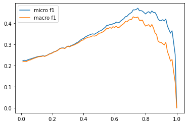
best_t,best_micro=thresholds[np.argmax(micros)],np.max(micros)(f'Best threshold (micro): {best_t} with F1-score {best_micro:.2f}.')best_t,best_macro=thresholds[np.argmax(macros)],np.max(macros)(f'Best threshold (micro): {best_t} with F1-score {best_macro:.2f}.')
Best threshold (micro): 0.75 with F1-score 0.47.
Best threshold (micro): 0.72 with F1-score 0.43.
This approach fares somewhat worse than the top-1 results but we can see the precision/recall trade-off clearly in this graph. If we choose the threshold too small, then there are too many predictions which lead to a low precision. If we choose the threshold too high, then we will make hardly no predictions which produces a low recall. From the plot we see that a threshold value of around 0.8 finds the sweet spot between the two.
Since the top-1 method performs best, let’s use this to compare zero-shot classification against Naive Bayes on the test set:
ds_zero_shot=ds['test'].map(zero_shot_pipeline)ds_zero_shot=ds_zero_shot.map(get_preds,fn_kwargs={'topk':1})clf_report=get_clf_report(ds_zero_shot)fortrain_sliceintrain_slices:macro_scores['Zero Shot'].append(clf_report['macro avg']['f1-score'])micro_scores['Zero Shot'].append(clf_report['micro avg']['f1-score'])
plot_metrics(micro_scores,macro_scores,train_samples,"Zero Shot")

Comparing the zero-shot pipeline to the baseline we observe two things:
-
If we have less than 50 labeled samples, the zero-shot pipeline handily outperforms the baseline.
-
Even above 50 samples, the performance of the zero-shot pipeline is superior when considering both the micro and macro
Note
You might notice a slight paradox in this section: although we talk about dealing with no labels, we still use the validation and test set. We use them to show-case different techniques and to make the results comparable between them. Even in a real use cas,e it makes sense to gather a handful of labeled examples to run some quick evaluations. The important point is that we did not adapt the parameters of the model with the data; instead we just adapted some hyperparameters.
If you find it difficult to get good results on your own dataset, here’s a few things you can do to improve the zero-shot pipeline:
-
The way the pipeline works makes it very sensitive to the names of the labels. If the names don’t make much sense or are not easily connected to the texts, the pipeline will likely perform poorly. Either try using different names or use several names in parallel and aggregate them in an extra step.
-
Another thing you can improve is the form of the hypothesis. By default it is “hypothesis=This is example is about {}“, but you can pass any other text to the pipeline. Depending on the use-case this might improve the performance as well.
Let’s now turn to the regime where we have a few labeled examples we can use to train a model.
Working With A Few Labels
In most NLP projects, you’ll have access to at least a few labelled examples. The labels might come directly from a client or cross-company team, or you might decide to just sit down and annotate a few examples yourself. Even for the previous approach we needed a few labelled examples to evaluate how well the zero-shot approach works. In this section, we’ll have a look at how we can best leverage the few, precious labelled examples that we have. Let’s start by looking at a technique known as data augmentation which can help multiply the little labelled data that we have.
Data Augmentation
One simple, but effective way to boost the performance of text classifiers on small datasets is to apply data augmentation techniques to generate new training examples from the existing ones. This is a common strategy in computer vision, where images are randomly perturbed without changing the meaning of the data (e.g. a slightly rotated cat is still a cat). For text, data augmentation is somewhat trickier because perturbing the words or characters can completely change the meaning. For example, the two questions “Are elephants heavier than mice?” and “Are mice heavier than elephants?” differ by a single word swap, but have opposite answers. However, if the text consists of more than a few sentences (like our GitHub issues do), then the noise introduced by these types of transformations will generally preserve the meaning of the label. In practice, there are two types of data augmentation techniques that are commonly used:
- Back translation
-
Take a text in the source language, translate it into one or more target languages using machine translation, and then translate back to the source language. Back translation tends to works best for high-resource languages or corpora that don’t contain too many domain-specific words.
- Token perturbations
-
Given a text from the training set, randomly choose and perform simple transformations like random synonym replacement, word insertion, swap, or deletion.6
An example of these transformations is shown in Table 5-1 and for a detailed list of other data augmentation techniques for NLP, we recommend reading A Visual Survey of Data Augmentation in NLP.
| Augmentation | Sentence |
|---|---|
None |
Even if you defeat me Megatron, others will rise to defeat your tyranny |
Synonym replace |
Even if you kill me Megatron, others will prove to defeat your tyranny |
Random insert |
Even if you defeat me Megatron, others humanity will rise to defeat your tyranny |
Random swap |
You even if defeat me Megatron, others will rise defeat to tyranny your |
Random delete |
Even if you me Megatron, others to defeat tyranny |
Backtranslate (German) |
Even if you defeat me, others will rise up to defeat your tyranny |
You can implement back translation using machine translation models like M2M100, while libraries like NlpAug and TextAttack provide various recipes for token perturbations. In this section, we’ll focus on using synonym replacement as it’s simple to implement and gets across the main idea behind data augmentation.
We’ll use the ContextualWordEmbsAug augmenter from NlpAug
to leverage the contextual word embeddings of DistilBERT for our synonym
replacements. Let’s start with a simple example:
fromtransformersimportset_seedimportnlpaug.augmenter.wordasnawset_seed(3)aug=naw.ContextualWordEmbsAug(model_path="distilbert-base-uncased",device="cpu",action="substitute")text="Transformers are the most popular toys"(f"Original text: {text}")(f"Augmented text: {aug.augment(text)}")
Original text: Transformers are the most popular toys
Augmented text: transformers represent the most popular toys
Here we can see how the word “are” has been replaced with “represent” to generate a new synthetic training example. We can wrap this augmentation in a simple function as follows:
defaugment_text(batch,transformations_per_example=1):text_aug,label_ids=[],[]fortext,labelsinzip(batch["text"],batch["label_ids"]):text_aug+=[text]label_ids+=[labels]for_inrange(transformations_per_example):text_aug+=[aug.augment(text)]label_ids+=[labels]return{"text":text_aug,"label_ids":label_ids}
Now when we call this function with Dataset.map we can generate any
number of new examples with the transformations_per_example argument.
We can use this function in our code to train the Naive Bayes classifier
by simply adding one line after we select the slice:
ds_train_sample=ds_train_sample.map(augment_text,batched=True,remove_columns=ds_train_sample.column_names).shuffle(seed=42)
Including this and re-running the analysis produces the plot shown below.
plot_metrics(micro_scores,macro_scores,train_samples,"Naive Bayes + Aug")

From the figure we can see that a small amount of data augmentation
improves the performance of the Naive Bayes classifier by around 5
points in
Using Embeddings as a Lookup Table
Large language models such as GPT-3 have been shown to be excellent at solving tasks with limited data. The reason is that these models learn useful representations of text that encode information across many dimensions such as sentiment, topic, text structure, and more. For this reason, the embeddings of large language models can be used to develop a semantic search engine, find similar documents or comments, or even classify text.
In this section we’ll create a text classifier that’s modeled after the OpenAI API classification endpoint. The idea follows a three step process:
-
Use the language model to embed all labeled texts.
-
Perform a nearest neighbor search over the stored embeddings.
-
Aggregate the labels of the nearest neighbors to get a prediction.
The process is illustrated in Figure 5-4.

Figure 5-4. An illustration of how nearest neighbour embedding lookup works: All labelled data is embedded with a model and stored with the labels. When a new text needs to be classified it is embedded as well and the label is given based on the labels of the nearest neighbours. It is important to calibrate the number of neighbours to be searched as too few might be noisy and too many might mix in neighbouring groups.
The beauty of this approach is that no model fine-tuning is necessary to leverage the few available labelled data points. Instead the main decision to make this approach work is to select an appropriate model that is ideally pretrained on a similar domain to your dataset.
Since GPT-3 it is only available through the OpenAI API, we’ll use GPT-2 to test the technique. Specifically, we’ll use a variant of GPT-2 that was trained on Python code, which will hopefully capture some of the context contained in our GitHub issues.
Let’s write a helper function that takes a list of texts and gets the vector representation using the model. We’ll take the last hidden state for each token and then calculate the average over all hidden states that are not masked:
importtorchfromtransformersimportAutoTokenizer,AutoModelmodel_ckpt="miguelvictor/python-gpt2-large"tokenizer=AutoTokenizer.from_pretrained(model_ckpt)model=AutoModel.from_pretrained(model_ckpt)defmean_pooling(model_output,attention_mask):token_embeddings=model_output[0]input_mask_expanded=(attention_mask.unsqueeze(-1).expand(token_embeddings.size()).float())sum_embeddings=torch.sum(token_embeddings*input_mask_expanded,1)sum_mask=torch.clamp(input_mask_expanded.sum(1),min=1e-9)returnsum_embeddings/sum_maskdefget_embeddings(text_list):encoded_input=tokenizer(text_list,padding=True,truncation=True,max_length=128,return_tensors="pt")withtorch.no_grad():model_output=model(**encoded_input)returnmean_pooling(model_output,encoded_input["attention_mask"])
Now we can get the embeddings for each split. Note that GPT-style models don’t have a padding token and therefore we need to add one before we can get the embeddings in a batched fashion as implemented above. We’ll just recycle the end-of-string token for this purpose:
text_embeddings={}tokenizer.pad_token=tokenizer.eos_tokenforsplitin["train","valid","test"]:text_embeddings[split]=get_embeddings(ds[split]["text"])
Now that we have all the embeddings we need to set up a system to search
them. We could write a function that calculates say the cosine
similiarity between a new text embedding that we’ll query
and the existing embeddings in the train set. Alternatively, we can use
a built-in structure of the Datasets library that is called a FAISS
index. You can think of this as a search engine for embeddings and
we’ll have a closer look how it works in a minute. We can
either use an existing field of the dataset to create a FAISS index with
Dataset.add_faiss_index or we can load new embeddings into the dataset
with Dataset.add_faiss_index_from_external_arrays. Let’s
use the latter function to add our train embeddings to the dataset as
follows:
ds["train"].add_faiss_index_from_external_arrays(np.array(text_embeddings["train"]),"embedding")
This created a new FAISS index called embedding. We can now perform a
nearest neighbour lookup by calling the function get_nearest_examples.
It returns the closest neighbours as well as the score matching score
for each neighbour. We need to specify the query embedding as well as
the number of nearest neighbours to retrieve. Let’s give it
a spin and have a look at the documents that are closest to an example:
query=np.array(text_embeddings['valid'][0],dtype=np.float32)k=3('label:',ds['valid'][0]['labels'])('text',ds['valid'][0]['text'][:200],'[...]')()('='*50)scores,samples=ds['train'].get_nearest_examples('embedding',query,k=k)('RETRIEVED DOCUMENTS:'+'='*50)forscore,label,textinzip(scores,samples['labels'],samples['text']):('TEXT:',text[:200],'[...]')('SCORE:',score)('LABELS:',label)('='*50)
Nice! This is exactly what we hoped for: the three retrieved documents
that we got via embedding lookup all have the same label and we can
already from the titles that they are all very similar. The question
remains, however, what is the best value for get_nearest_examples_batch which allows as to retrieve
documents for a batch of queries:
max_k=17perf_micro=np.zeros((max_k,max_k))perf_macro=np.zeros((max_k,max_k))defget_sample_preds(sample,m):return(np.sum(sample["label_ids"],axis=0)>=m).astype(int)forkinrange(1,max_k):forminrange(1,k+1):query_batch=np.array(text_embeddings["valid"],dtype=np.float32)scores,samples=ds["train"].get_nearest_examples_batch("embedding",query_batch,k=k)y_pred=np.array([get_sample_preds(sample,m)forsampleinsamples])clf_report=classification_report(np.array(ds["valid"]["label_ids"]),y_pred,target_names=mlb.classes_,zero_division=0,output_dict=True)perf_micro[k,m]=clf_report["micro avg"]["f1-score"]perf_macro[k,m]=clf_report["macro avg"]["f1-score"]

From the plots we can see that the performance is best when we choose
k,m=7,3ds["train"].drop_index("embedding")fortrain_sliceintrain_slices:ds_train=ds["train"].select(train_slice)emb_slice=np.array(text_embeddings["train"])[train_slice]ds_train.add_faiss_index_from_external_arrays(emb_slice,"embedding")query_batch=np.array(text_embeddings["test"],dtype=np.float32)scores,samples=ds_train.get_nearest_examples_batch("embedding",query_batch,k=k)y_pred=np.array([get_sample_preds(sample,m)forsampleinsamples])clf_report=classification_report(np.array(ds["test"]["label_ids"]),y_pred,target_names=mlb.classes_,zero_division=0,output_dict=True,)macro_scores["Embedding"].append(clf_report["macro avg"]["f1-score"])micro_scores["Embedding"].append(clf_report["micro avg"]["f1-score"])
plot_metrics(micro_scores,macro_scores,train_samples,"Embedding")

These results look promising: the embedding lookup beats the Naive Bayes baseline with 32 samples in the training set. Although we don’t manage to beat the zero-shot pipeline on the macro scores until around 100 examples. That means for this use-case if you have fewer than 32 samples it makes sense to give the zero-shot pipeline a shot and if you have more samples you could give an embedding lookup a shot. If it is more important to perform well on all classes equally you might be better off with the zero-shot pipeline until you have more than 100 labels.
Take these results with a grain of salt; which method works best
strongly depends on the domain. The zero-shot pipeline’s
training data is quite different from the GitHub issues
we’re using it on which contains a lot of code which the
model likely has not encountered much before. For a more common task
such as sentiment analysis of reviews the pipeline might work much
better. Similarly, the embeddings’ quality depends on the
model and data it was trained on. We tried half a dozen models such as
'sentence-transformers/stsb-roberta-large'
which was trained to give high quality embeddings of sentences, and
'microsoft/codebert-base' as well as
'dbernsohn/roberta-python' which were trained
on code and documentation. For this specific use-case GPT-2 trained on
Python code worked best.
Since you don’t actually need to change anything in your code besides replacing the model checkpoint name to test another model you can quickly try out a few models once you have the evaluation pipeline setup. Before we continue the quest of finding the best approach in the sparse label domain we want to take a moment to spotlight the FAISS library.
Efficient Similarity Search With FAISS
We first encountered FAISS in Chapter 2 where we used it to retrieve documents via the DPR embeddings. Here we’ll explain briefly how the FAISS library works and why it is a powerful tool in the ML toolbox.
We are used to performing fast text queries on huge datasets such as Wikipedia or the web with search engines such as Google. When we move from text to embeddings we would like to maintain that performance; however, the methods used to speed up text queries don’t apply to embeddings.
To speed up text search we usually create an inverted index that maps terms to documents. An inverted index works like an index at the end of a book: each word is mapped to the pages (or in our case document) it occurs in. When we later run a query we can quickly look up in which documents the search terms appear. This works well with discrete objects such as words but does not work with continuous objects such as vectors. Each document has likely a unique vector and therefore the index would never match with a new vector. Instead of looking for exact matches we need to look for close or similar matches.
When we want to find the most similar vectors in a database to a query vector in theory we would need to compare the query vector to each vector in the database. For a small database such as we have in this chapter this is no problem but when we scale this up to thousands or even million of entries we would need to wait for a while until a query is processed.
FAISS addresses this issues with several tricks. The main idea is to
partition the dataset. If we only need to compare the query vector to a
subset of the database we can speed up the process significantly. But if
we just randomly partition the dataset how could we decide which
partition to search and what guarantees do we get for finding the most
similar entries. Evidently, there needs to be a better solution: apply

Figure 5-5. This figure depicts the structure of a FAISS index. The grey points represent data points added to the index and the bold black points are the cluster centeres found via k-means clustering. The colored areas represent the regions belonging to a cluster center.
Given such a grouping, search is much easier: we first search across the
centroids for the one that is most similar to our query and then we
search within the group. This reduces the number of comparisons from

In the plot you can see the number of comparisons as a function of the
number of clusters. We are looking for the minimum of this function
where we need to do the least comparisons. We can see that the minimum
is exactly where we expected to see at
In addition to speeding up queries with partitioning, FAISS also allows you to utilize GPUs for further speedup. If memory becomes a concern there are also several options to compress the vectors with advanced quantization schemes. If you want to use FAISS for your project the repository has a simple guide for you to choose the right methods for your use-case.
One of the largest projects to use FAISS was the creation of the CCMatrix corpus by Facebook. They used multilingual embeddings to find parallel sentences in different languages. This enormous corpus was subsequently used to train M2M-100, a large machine translation model that is able to directly translate between any of 100 languages.
That was a little detour through the FAISS library. Let’s get back to classification now and have a stab at fine-tuning a transformer on a few labelled examples.
Fine-tuning a Vanilla Transformer
If we have access to labeled data we can also try to do the obvious
thing: simply fine-tune a pretrained transformer model. We can either
use a standard checkpoint such as bert-base-uncased or we can also try
a checkpoint of a model that has been specifically tuned on a domain
closer to ours such as giganticode/StackOBERTflow-comments-small-v1
that has been trained on discussions on Stack
Overflow. In general, it can make a lot of sense to use a model that is
closer to your domain and there are over 10,000 models available on the
Hugging Face hub. In our case, however, we found that the standard BERT
checkpoint worked best.
Let’s start by loading the pretrained tokenizer and tokenize our dataset and get rid of the columns we don’t need for training and evaluation:
fromtransformersimport(AutoTokenizer,AutoConfig,AutoModelForSequenceClassification)model_ckpt="bert-base-uncased"tokenizer=AutoTokenizer.from_pretrained(model_ckpt)deftokenize(batch):returntokenizer(batch["text"],truncation=True,max_length=128)ds_enc=ds.map(tokenize,batched=True)ds_enc=ds_enc.remove_columns(['labels','text'])
One thing that is special about our use-case is the multilabel
classification aspect. The models and Trainer don’t
support this out of the box but the Trainer can be easily modified for
the task. Part of the Trainer’s training loop is the call
to the compute_loss function which returns the loss. By subclassing
the Trainer and overwriting the compute_loss function we can adapt
the loss to the multilabel case. Instead of calculating the
cross-entropy loss across all labels we calculate it for each output
class separately. We can do this by using the
torch.nn.BCEWithLogitsLoss function:
fromtransformersimportTrainer,TrainingArgumentsimporttorchclassMultiLabelTrainer(Trainer):defcompute_loss(self,model,inputs,return_outputs=False):num_labels=self.model.config.num_labelslabels=inputs.pop("labels")outputs=model(**inputs)logits=outputs.logitsloss_fct=torch.nn.BCEWithLogitsLoss()loss=loss_fct(logits.view(-1,num_labels),labels.type_as(logits).view(-1,num_labels))return(loss,outputs)ifreturn_outputselseloss
Since we are likely to quickly overfit the training data due to its
limited size we set the load_best_model_at_end=True and choose the
best model based on the micro F1-score.
training_args_fine_tune=TrainingArguments(output_dir="./results",num_train_epochs=20,learning_rate=3e-5,lr_scheduler_type='constant',per_device_train_batch_size=4,per_device_eval_batch_size=128,weight_decay=0.0,evaluation_strategy="epoch",logging_steps=15,save_steps=-1,load_best_model_at_end=True,metric_for_best_model='micro f1',report_to="none")
Since we need the F1-score to choose the best model we need to make sure it is calculated during the evaluation. Since the model returns the logits we first need to normalize the predictions with a sigmoid function and can then binarize them with a simple threshold. Then we return the scores we are interested in from the classification report:
fromscipy.specialimportexpitassigmoiddefcompute_metrics(pred):y_true=pred.label_idsy_pred=sigmoid(pred.predictions)y_pred=(y_pred>0.5).astype(float)clf_dict=classification_report(y_true,y_pred,target_names=all_labels,zero_division=0,output_dict=True)return{"micro f1":clf_dict['micro avg']['f1-score'],"macro f1":clf_dict['macro avg']['f1-score']}
Now we are ready to rumble! For each training set slice we train a classifier from scratch, load the best model at the end of the training loop and store the results on the test set:
config=AutoConfig.from_pretrained(model_ckpt)config.num_labels=len(all_labels)fortrain_sliceintrain_slices:model=AutoModelForSequenceClassification.from_pretrained(model_ckpt,config=config)trainer=MultiLabelTrainer(model=model,tokenizer=tokenizer,args=training_args_fine_tune,compute_metrics=compute_metrics,train_dataset=ds_enc["train"].select(train_slice),eval_dataset=ds_enc["valid"],)trainer.train()pred=trainer.predict(ds_enc['test'])metrics=compute_metrics(pred)macro_scores['Fine-tune (vanilla)'].append(metrics['macro f1'])micro_scores['Fine-tune (vanilla)'].append(metrics['micro f1'])
plot_metrics(micro_scores,macro_scores,train_samples,"Fine-tune (vanilla)")

First of all we see that simply fine-tuning a vanilla BERT model on the dataset leads to competitive results when we have access to around 64 examples. We also see that before the behavior is a bit erratic which is again due training a model on a small sample where some labels can be unfavorably unbalanced. Before we make use of the unlabeled part of our dataset let’s take a quick look at another promising approach for using language models in the few-shot domain.
In-context and Few-shot Learning with Prompts
We’ve seen in the zero-shot classification section that we can use a language model like BERT or GPT-2 and adapt it to a supervised task by using prompts and parsing the model’s token predictions. This is different from the classical approach of adding a task specific head and tuning the model parameters for the task. On the plus side this approach does not require any training data but on the negative side it seems we can’t levarage labeled data if we have access to it. There is a middle ground sometimes called in-context or few-shot learning.
To illustrate the concept, consider a English to French translation task. In the zero-shot paradigm we would construct a prompt that might look as follows:
prompt="""Translate English to German:thanks =>"""
This hopefully prompts the model to predict the tokens of the word “merci”. The clearer the task the better this approach works. An interesting finding of the GPT-3 paper7 was the ability of the model to effectively learn from examples presented in the prompt. What OpenAI found is that you can improve the results by adding examples of the task to the prompt as illustrated in figure Figure 5-6.
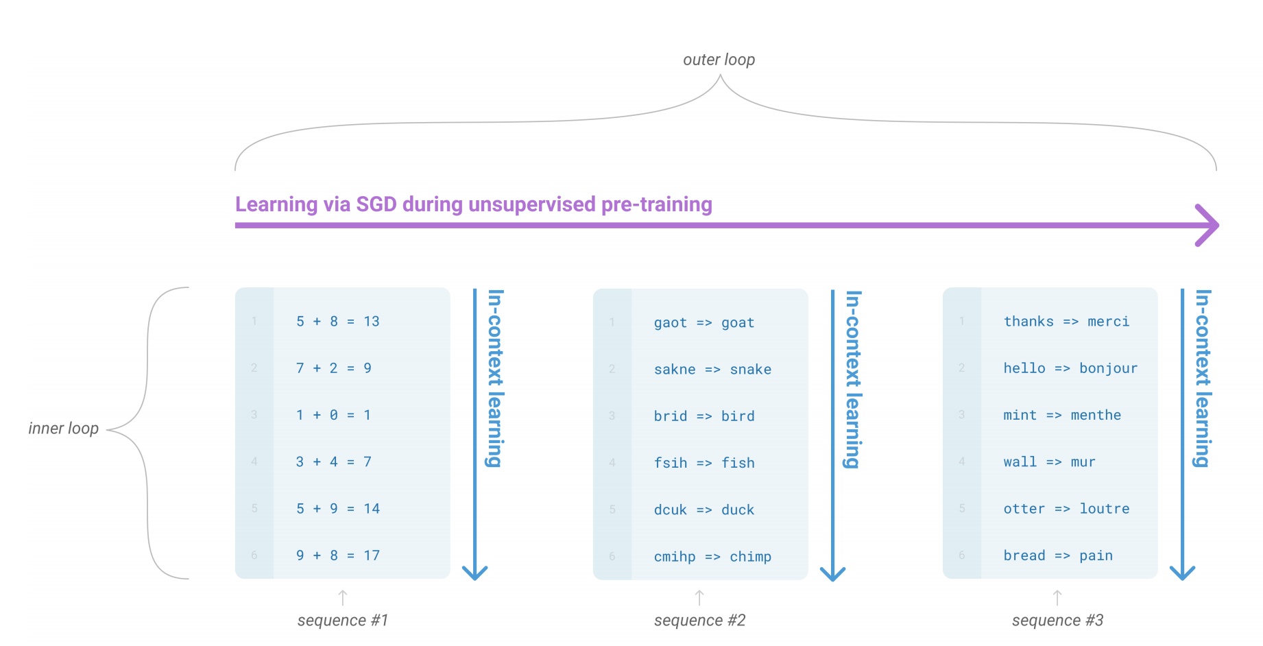
Figure 5-6. This figure illustrate how GPT-3 can utilize examples of the task provieded in the context. Such sequences of examples can occur naturally in the pretraining corpus and thus the model learns to interpret such sequences to better predict the next token. Image from Language Models are Few-Shot Learners by T. Brown et al (2020).
Furthermore, they found that the larger the models are scaled the better they are at using the in-context examples leading to significant performance boosts. Although GPT-3 sized models are challenging to use in production, this is an exciting emerging research field and people have built cool applications such as a natural language shell where commands are entered in natural language and parsed by GPT-3 to shell commands.
An alternative approach to use labeled data is to create examples of the prompts and desired predictions and continue training the language model on these examples. A novel method called ADAPET8 uses such an approach and beats GPT-3 on a wide variety of task tuning the model with generated prompts. Recent work by Hugging Face researchers9 suggests that such an approach can be more data efficient than fine-tuning a custom head.
In this section we looked at various ways to make good use of the few labelled examples that we have. Very often we also have access to a lot of unlabelled data in addition to the labelled examples and in the next section we have a look at how to make good use of it.
Levaraging Unlabelled Data
Although large volumes of high-quality labeled data is the best case scenario to train a classifier, this does not mean that unlabeled data is worthless. Just think about the pretraining of most models we have used: even though they are trained on mostly unrelated data from the internet, we can leverage the pretrained weights for other tasks on wide variety of texts. This is the core idea of transfer learning in NLP. Naturally, if the downstream tasks has similar textual structure as the pretraining texts the transfer works better. So if we can bring the pretraining task closer to the downstream objective we could potentially improve the transfer.
Let’s think about this in terms of our concrete use-case: BERT is pretrained on the Book Corpus and English Wikipedia so texts containing code and GitHub issues are definitely a small niche in these dataset. If we pretrained BERT from scratch we could do it on a crawl of all of the issues on GitHub for example. However, this would be expensive and a lot of aspects about language that BERT learned are still valid for GitHub issues. So is there a middle-ground between retraining from scratch and just use the model as is for classification? There is and it is called domain adaptation. Instead of retraining the language model from scratch we can continue training it on data from our domain. In this step we use the classical language model objective of predicting masked words which means we don’t need any labeled data for this step. After that we can then load the adapted model as a classifier and fine-tune it, thus leveraging the unlabeled data.
The beauty of domain adaptation is that compared to labeled data, unlabeled data is often abundantly available. Furthermore, the adapted model can be reused for many use-cases. Imagine you want to build an email classifier and apply domain adaptation on all your historic emails. You can later use the same model for named entity recognition or another classification task like sentiment analysis, since the approach is agnostic to the downstream task.
Fine-tuning a Language Model
In this section we’ll fine-tune the pretrained BERT model with masked language modeling on the unlabeled portion of the dataset. To do this we only need two new concepts: an extra step when tokenizing the data and a special data collator. Let’s start with the tokenization.
In addition to the ordinary tokens from the text the tokenizer also adds
special tokens to the sequence such as the [CLS] and the [SEP] token
which are used for classification and next sentence prediction. When we
do masked language model we want to make sure we don’t train
the model to also predict these tokens. For this reason we mask them
from the loss and we can get a mask when tokenizing by setting
return_special_tokens_mask=True. Let’s re-tokenize the
text with that setting:
fromtransformersimportDataCollatorForLanguageModeling,BertForMaskedLM
deftokenize(batch):returntokenizer(batch["text"],truncation=True,max_length=128,return_special_tokens_mask=True)ds_mlm=ds.map(tokenize,batched=True)ds_mlm=ds_mlm.remove_columns(['labels','text','label_ids'])
What’s missing to start with masked language modeling is the mechanism to mask tokens in the input sequence and have the target tokens in the outputs. One way we could approach this is by setting up a function that masks random tokens and creates labels for these sequences. On the one hand this would double the size of the dataset since we would also store the target sequence in the dataset and on the other hand we would use the same masking of a sequence every epoch.
A much more elegant solution to this is the use of a a data collator.
Remember that the data collator is the function that builds the bridge
between the dataset and the model calls. A batch is sampled from the
dataset and the data collator prepares the elements in the batch to feed
them to the model. In the simplest case we have encountered it simply
concatenates the tensors of each element into a a single tensor. In our
case we can use it to do the masking and label generation on the fly.
That way we don’t need to store it and we get new masks
everytime we sample. The data collator for this task is called
DataCollatorForLanguageModeling and we initialize it with the
model’s tokenizer and the fraction of tokens we want to
masked called mlm_probability. We use this collator to mask 15% of the
tokens which follows the procedure in the original BERT paper:
data_collator=DataCollatorForLanguageModeling(tokenizer=tokenizer,mlm_probability=0.15)
With the tokenizer and data collator in place we are ready to fine-tune the masked language model. We chose the batch size to make most use of the GPUs, but you may want to reduce it if you run into out-of-memory errors:
training_args=TrainingArguments(output_dir=f'./models/{model_ckpt}-issues-128',per_device_train_batch_size=64,evaluation_strategy='epoch',num_train_epochs=16,save_total_limit=5,logging_steps=15,report_to="none")trainer=Trainer(model=BertForMaskedLM.from_pretrained('bert-base-uncased'),args=training_args,train_dataset=ds_mlm["unsup"],eval_dataset=ds_mlm['train'],tokenizer=tokenizer,data_collator=data_collator,)trainer.train()
trainer.model.save_pretrained(training_args.output_dir)
We can access the trainer’s log history to look at the
training and validation losses of the model. All logs are stored in
trainer.state.log_history as a list of dictionaries which we can
easily load into a Pandas DataFrame. Since the validation is not
performed in sync with the normal loss calculation there are missing
values in the dataframe. For this reason we drop the missing values
before plotting the metrics:
importpandasaspddf_log=pd.DataFrame.from_records(trainer.state.log_history)df_log.dropna(subset=['eval_loss'])['eval_loss'].plot(title='loss')df_log.dropna(subset=['loss'])['loss'].plot();
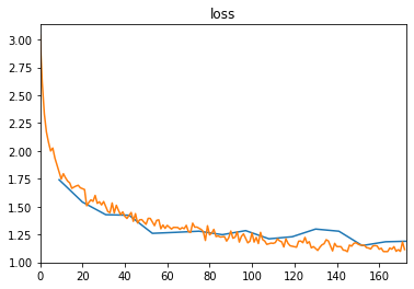
It seems that both the training and validation loss went down considerably. So let’s check if we can also see an improvement when we fine-tune a classifier based on this model.
Fine-tuning a Classifier
Now we repeat the fine-tuning procedure with the slight difference that we load our own, custom checkpoint:
model_ckpt=f'./models/bert-base-uncased-issues-128'config=AutoConfig.from_pretrained(model_ckpt)config.num_labels=len(all_labels)fortrain_sliceintrain_slices:model=AutoModelForSequenceClassification.from_pretrained(model_ckpt,config=config)trainer=MultiLabelTrainer(model=model,tokenizer=tokenizer,args=training_args_fine_tune,compute_metrics=compute_metrics,train_dataset=ds_enc["train"].select(train_slice),eval_dataset=ds_enc["valid"],)trainer.train()pred=trainer.predict(ds_enc['test'])metrics=compute_metrics(pred)macro_scores['Fine-tune (DA)'].append(metrics['macro f1'])micro_scores['Fine-tune (DA)'].append(metrics['micro f1'])
Comparing the results to the fine-tuning based on vanilla BERT we see that we get an advantage especially in the low data domain but also when we have access to more labels we get at least a few percent gain:
plot_metrics(micro_scores,macro_scores,train_samples,"Fine-tune (DA)")

This highlights that domain adaptation can improve the model performance with unlabeled data and little effort. Naturally the more unlabeled data and the fewer labeled data you have the more impact you will get with this method. Before we conclude this chapter we want to show two methods how you can leverage the unlabeled data even further with a few tricks.
Advanced Methods
Fine-tuning the language model before tuning it is a nice method since it is straightforward and yields reliable performance boosts. However, there are a few more sophisticated methods than can leverage unlabeled data even further. Showcasing these methods is beyond the scope of this book but we summarize them here which should give a good starting point should you need more performance.
Universal Data Augmentation
The first method is called universal data augmentation (UDA) and describes an approach to use unlabeled data that is not only limited to text. The idea is that a model’s predictions should be consistent even if the input is slightly distorted. Such distortions are introduced with standard data augmentation strategies: rotations and random noise for images and token replacements and back-translations with text. We can enforce consistency by creating a loss term based on the KL-divergence between the predictions of the original and distorted input.
The interesting aspect is that we can enforce the consistency on the unlabeled data and even though we don’t know what the correct prediction is we minimize the KL-divergence between the predictions. So on the one hand we train the labeled data with the standard supervised approach and on the other hand we introduce a second training loops where we train the model to make consistent predictions on the unlabeled data as outlined in figure Figure 5-7.
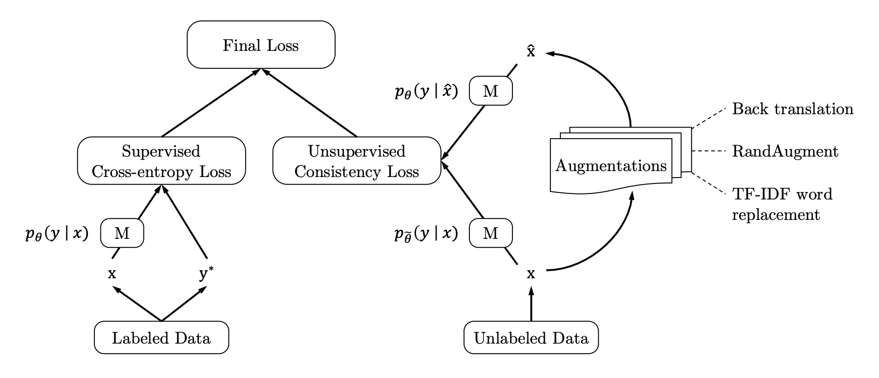
Figure 5-7. With UDA the classical cross-entropy loss from the labelled samples is augmented with the consistency loss from unlabelled samples. Image from the UDA paper.
The performance of this approach with a handful of labels gets close to the performance with thousands of examples. The downside is that you first need an data augmentation pipeline and then training takes much longer since you also train on the unlabeled fraction of your dataset.
Uncertainty-Aware Self-Training
Another, promising method to leverage unlabeled data is Uncertainty-aware Self-training (UST). The idea is to train a teacher model on the labeled data and then use that model to create pseudo-labels on the unlabeled data. Then a student is trained on the pseudo-labeled data and after training becomes the teacher for the next iteration.
One interesting aspect of this method is how the pseudo-labels are generated: to get an uncertainty measure of the model’s predictions the same input is fed several times through the model with dropout turned on. Then the variance in the predictions give a proxy for the certainty of the model on a specific sample. With that uncertainty measure the pseudo-labels are then sampled using a method called Bayesian Active Learning by Disagreement (BALD). The full training pipeline is illustrated in Figure 5-8.

Figure 5-8. The UST method consists of a teacher that generated pseudo labels and a student that is subsequently trained on those labels. After the student is trained it becomes the teacher and the step is repeated. Image from the UST paper.
With this iteration scheme the teacher continuously gets better at creating pseudo-labels and thus the model improves performance. In the end this approach also gets within a few percent of model’s trained on the full training data with thousands of samples and even beats UDA on several datasets. This concludes the this section on leveraging unlabeled data and we now turn to the conclusion.
Conclusion
In this chapter we’ve seen that even if we have only a few or even no labels that not all hope is lost. We can utilize models that have been pretrained on other tasks such as the BERT language model or GPT-2 trained on Python code to make predictions on the new task of GitHub issue classification. Furthermore, we can use domain adaptation to get an additional boost when training the model with a normal classification head.
Which of the presented approaches work best on a specific use-case depend on a variety of aspects: how much labeled data do you have, how noisy is it, how close is the data to the pretraining corpus and so on. To find out what works best it is a good idea to setup an evaluation pipeline and then iterate quickly. The flexible transformer library API allows you to quickly load a handful of models and compare them without the need for any code changes. There are over 10,000 on the model hub and chances are somebody worked on a similar problem in a past and you can build on top of this.
One aspect that is beyond this book is the trade-off between a more complex approach like UDA or UST and getting more data. To evaluate your approach it makes sense to at least build a validation and test set early on. At every step of the way you can also gather more labeled data. Usually annotating a few hundred examples is a matter of a couple hours or a few days and there are many tools that assist you doing so. Depending on what you are trying to achieve it can make sense to invest some time creating a small high quality dataset over engineering a very complex method to compensate for the lack thereof. With the the methods we presented in this notebook you can ensure that you get the most value out of your precious labeled data.
All the tasks that we’ve seen so far in this book fall in the domain of natural language understanding (NLU), where we have a text as an input and use it to make a some sort of classification. For example, in text classification we predicted a single class for an input sequence, while in NER we predicted a class for each token. In question-answering we classified each token as a start or end token of the answer span. We now turn from NLU tasks to natural language generation (NLG) tasks, where both the input and the output consist of text. In the next chapter we explore how to train models for summarization where the input is a long texts and the output is a short text with its summary.
1 Unsupervised Data Augmentation for Consistency Training, Q. Xie et al. (2019)
2 Uncertainty-Aware Self-Training for Few-Shot Text Classification, S. Mukherjee et al. (2020)
3 We thank Joe Davison for suggesting this approach to us.
4 A Broad-Coverage Challenge Corpus for Sentence Understanding through Inference, A. Williams et al. (2018)
5 XNLI: Evaluating Cross-lingual Sentence Representations, A. Conneau et al. (2018)
6 EDA: Easy Data Augmentation Techniques for Boosting Performance on Text Classification Tasks, J. Wei and K. Zou (2019)
7 Language Models are Few-Shot Learners, T. Brown et al. (2020)
8 Improving and Simplifying Pattern Exploiting Training, D. Tam et al. (2021)
9 How Many Data Points is a Prompt Worth?, T. Le Scao (2021)