Uncertainty

Consider an economy with a general, discrete state space $\Omega$ with a finite number of elements $\left|\Omega \right|<\infty$. An algebra $ℱ$ in $\Omega$ is a family of sets for which the following statements hold true:

1. $\Omega \in ℱ$

2. $?\in ℱ\Rightarrow {?}^c\in ℱ$

3. ${?}_1,{?}_2,...,{?}_I\in ℱ\Rightarrow {\cup }_{i=1}^I{?}_i\in ℱ$

${?}^c$ denotes the complement of a set $?$. The power set $\wp \left(\Omega \right)$ is the largest algebra while the set $ℱ=\{\varnothing ,\Omega \}$ is the smallest algebra in $\Omega$. An algebra is a model for observable events in an economy. In this context, a single state of the economy $\omega \in \Omega$ can be interpreted as an atomic event.

A probability assigns a real number $0\le p_{\omega }\equiv P\left(\left\{\omega \right\}\right)\le 1$ to a state $\omega \in \Omega$ or a real number $0\le P\left(?\right)\le 1$ to an event $?\in ℱ$. If the probabilities for all states are known, one has $P\left(?\right)={\sum }_{\omega \in ?}{p}_{\omega }$.

A probability measure $P:ℱ\to [0,1]$ is characterized by the following characteristics:

1. $\forall ?\in ℱ:P\left(?\right)\ge 0$

2. $P\left({\cup }_{i=1}^I{?}_i\right)={\sum }_{i=1}^I{?}_i\text{for}\text{disjoint}\text{sets}{?}_i\in ℱ$

3. $P\left(\Omega \right)=1$

Together the three elements $\{\Omega ,ℱ,P\}$ form a probability space. A probability space is the formal representation for uncertainty in the model economy.

In [1]: import numpy as np
        np.set_printoptions(precision=5)

In [2]: np.random.seed(100)  

In [3]: I = 1000  

In [4]: S = np.random.normal(loc=100, scale=20, size=I)  

In [5]: S[:14]  
Out[5]: array([ 65.00469, 106.85361, 123.06072,  94.95128, 119.62642, 110.28438,
               104.42359,  78.59913,  96.21008, 105.10003,  90.83946, 108.70327,
                88.3281 , 116.33694])

In [6]: S.mean()  
Out[6]: 99.66455685312181

In [7]: P = np.random.random(I)  

In [8]: P[:10]  
Out[8]: array([0.079  , 0.36885, 0.0657 , 0.2236 , 0.25101, 0.94175, 0.1182 ,
               0.81407, 0.34056, 0.79935])

In [9]: P /= P.sum()  

In [10]: P.sum()  
Out[10]: 1.0

In [11]: P[:10]  
Out[11]: array([0.00017, 0.00077, 0.00014, 0.00047, 0.00053, 0.00197, 0.00025,
                0.00171, 0.00071, 0.00167])

In [12]: np.dot(P, S)  
Out[12]: 99.48909209680373

Financial Assets

Consider an economy at two different dates $t\in \{0,1\}$, today and one year from now (or any other time period in the future to this end). Assume that a probability space $\{\Omega ,ℱ\equiv \wp (\Omega ),P\}$ is given that represents uncertainty about the future in the model economy, with $\left|\Omega \right|\equiv I$ possible future states. In this case, $\Omega =\{{\omega }_1,{\omega }_2,...,{\omega }_I\}$.

A traded financial asset is represented by a price process $S=(S_0,S_1)$ where the price today is fixed $S_0\in {ℝ}_{>0}$ and the price in one year $S_1:\Omega \to {ℝ}_{\ge 0}$ is a random variable that is $ℱ-$measurable. Formally, the future price vector of a traded financial asset is a vector with $I$ elements

If there are multiple financial assets traded, say $K>1$, they are represented by multiple price processes $S^k=(S_0^k,S_1^k),k=1,2,...,K$. The market payoff matrix is then composed of the future price vectors of the traded financial assets.

Denote the set of traded financial assets by $?\equiv (S^1,S^2,...,S^K)$. The static model economy can then be summarized by

where it is usually assumed that $ℱ\equiv \wp \left(\Omega \right)$.

Fixing the number of possible future states to five $\Omega =\{{\omega }_1,...,{\omega }_5\}$ with equal probability $\forall \omega \in \Omega :P\left(\omega \right)=\frac{1}{5}$ and the number of traded financial assets to five as well, a numerical example in Python illustrates such a static model economy.

In [13]: M = np.array((
             (11, 25, 0,  0,  25),
             (11, 20, 30, 15, 25),
             (11, 10, 0,  20, 10),
             (11, 5,  30, 15, 0),
             (11, 0,  0,  0,  0)
         ))  

In [14]: M0 = np.array(5 * [10.])  

In [15]: M0  
Out[15]: array([10., 10., 10., 10., 10.])

In [16]: M.mean(axis=0)  
Out[16]: array([11., 12., 12., 10., 12.])

In [17]: mu = M.mean(axis=0) / M0 - 1  

In [18]: mu  
Out[18]: array([0.1, 0.2, 0.2, 0. , 0.2])

In [19]: (M / M0 - 1)  
Out[19]: array([[ 0.1,  1.5, -1. , -1. ,  1.5],
                [ 0.1,  1. ,  2. ,  0.5,  1.5],
                [ 0.1,  0. , -1. ,  1. ,  0. ],
                [ 0.1, -0.5,  2. ,  0.5, -1. ],
                [ 0.1, -1. , -1. , -1. , -1. ]])

In [20]: sigma = (M / M0 - 1).std(axis=0)  

In [21]: sigma  
Out[21]: array([0.     , 0.92736, 1.46969, 0.83666, 1.1225 ])

The assumed market payoff matrix where the columns represent the future, uncertain price vectors of the traded financial assets.

The current price vector for the five assets for each of which the price is fixed to 10.

This calculates the expected (or average) future price for every traded financial asset.

This in turn calculates the expected (or average) rates of return.

The rates of return matrix calculated and printed out.

The standard deviation of the rates of return or volatility calculated for every traded financial asset — the first one is risk-less, it can be considered to be a bond.

Contingent Claims

Given a model economy $ℰ$, a contingent claim is characterized by a price process $C=(C_0,C_1)$ where $C_1$ is a $ℱ-$measurable random variable.

One can think of European call and put options as canonical examples of contingent claims. The payoff of a European call option might, for instance, be defined relative to the second traded financial asset according to $C_1=max(S_1^2-K,0)$ where $K\in {ℝ}_{\ge 0}$ is the strike price of the option. Since the payoff of the option is “derived” from another asset, one therefore often speaks of derivative instruments or derivatives for short.

If a contingent claim can be replicated by a portfolio $\varphi \in {ℝ}^K$ of the traded financial assets $?$

then the arbitrage price of the contingent claim is

where ${ℳ}_{\mathcal{0}}={\left(S_0^1,S_0^2,...,S_0^K\right)}^T\in {ℝ}_{++}^I$ is the current price vector of the traded financial assets.

Continuing the Python example from before, replication of contingent claims based on linear algebra methods is illustrated in the following.

In [22]: K = 15  

In [23]: M[:, 1]  
Out[23]: array([25, 20, 10,  5,  0])

In [24]: C1 = np.maximum(M[:, 1] - K, 0)  

In [25]: C1  
Out[25]: array([10,  5,  0,  0,  0])

In [26]: phi = np.linalg.solve(M, C1)  

In [27]: phi  
Out[27]: array([-9.08364e-17,  5.00000e-01,  1.66667e-02, -2.00000e-01,
                -1.00000e-01])

In [28]: C1 == np.dot(M, phi)  
Out[28]: array([ True, False, False, False, False])

In [29]: C0 = np.dot(M0, phi)  

In [30]: C0  
Out[30]: 2.1666666666666665

The strike price of the European call option and the payoff vector of the relevant financial asset.

The call option is written on the second traded financial asset with future payoff of $S_1^2=(25,20,10,5,0)$.

This solves the replication problem given the market payoff matrix.

Checks whether the replication portfolio indeed perfectly replicates the future payoff of the European call option.

From the replication portfolio, the arbitrage price follows in combination with the current price vector of the traded financial assets.

Market Completeness

Market completeness of the static model economy can be analyzed based on the rank of the market payoff matrix $ℳ$ as defined by the traded financial assets $?$. The rank of a matrix equals the number of linearly independent (column or row) vectors (see Aleskerov et al. (2011), sec. 2.7). Consider the column vectors that represent the future price vectors of the traded financial assets. They are linearly independent if

has only one solution, namely the null vector $\varphi ={(0,0,...,0)}^T\in {ℝ}^K$.

On the other hand, the span of the market payoff matrix $ℳ$ is given by all linear combinations of the column vectors

The model economy $ℰ$ is complete if the set of attainable contingent claims satisfies $?={ℝ}^I$. However, the set of attainable contingent claims equals by definition the span of the traded financial assets $?\equiv \text{span}\left(ℳ\right)$. The model economy $ℰ$ therefore is complete if

Under which circumstances is this the case? It is the case if the rank of the matrix is at least as large as the number of future states possible

In other words the column vectors of $ℳ$ form a basis of the vector space ${ℝ}^I$ (with potentially more basis vectors than required). A vector space $?$ is a set of elements (called vectors) that is characterized by

1. an addition function mapping two vectors $v_1,v_2\in ?$ to another element of the vector space $(v_1+v_2)\in ?$.

2. a scalar multiplication function mapping a scalar $\alpha \in ℝ$ and a vector $v\in ?$ to another element of the vector space $(\alpha ·v)\in ?$.

3. a special element — usually called “zero” or “netural element" — $0\in ?$ such that $v+0=v$

It is easy to verify that, for example, the sets $ℝ,{ℝ}^5$ or ${ℝ}^I,I\in {\mathbb{N}}_{+},$ are vector spaces.

Consequently, the model economy is incomplete if

To make things a bit more concrete, consider a state space with three possible future states only $\Omega =\{{\omega }_1,{\omega }_2,{\omega }_3\}$. All random variables then are vectors in the vector space ${ℝ}^3$. The following market payoff matrix — resulting from three traded financial assets — has a rank of 2 only since two column vectors are linearly dependent. This leads to an incomplete market.

It is easily verified that the financial assets 2 and 3 are indeed linearly dependent.

By contrast, the market payoff matrix below — resulting from a different set of three traded financial assets — has a rank of 3, leading to a complete market. In such a case, one also speaks of the matrix having full rank:

Assume next that a probability space is fixed for which the state space has five elements $\Omega =\{{\omega }_1,...,{\omega }_5\}$. The future (uncertain) price and payoff vectors of the five traded financial assets $?$ and all contingent claims, respectively, are now elements of the vector space ${ℝ}^5$. The Python that follows analyzes contingent claim replication based on such a model economy $ℰ$. It starts by assuming that all five Arrow-Debreu securities are traded and then proceeds to a randomized market payoff matrix.

In [31]: M = np.eye(5)  

In [32]: M  
Out[32]: array([[1., 0., 0., 0., 0.],
                [0., 1., 0., 0., 0.],
                [0., 0., 1., 0., 0.],
                [0., 0., 0., 1., 0.],
                [0., 0., 0., 0., 1.]])

In [33]: np.linalg.linalg.matrix_rank(M)  
Out[33]: 5

In [34]: C1 = np.arange(10, 0, -2)  

In [35]: C1  
Out[35]: array([10,  8,  6,  4,  2])

In [36]: np.linalg.solve(M, C1)  
Out[36]: array([10.,  8.,  6.,  4.,  2.])

Creates a two-dimensional ndarray object, here an identity matrix. It can be interpreted as the market payoff matrix resulting from five traded Arrow-Debreu securities. It forms a (so-called canonical) basis of the vector space ${ℝ}^5$.

Calculates the rank of the matrix which is trivial to see for the identity matrix.

A contingent claim payoff which is to be replicated by the traded financial assets.

This solves the replication (representation) problem which is again trivial in the case of the identity matrix.

Next, a randomized market payoff matrix is generated which happens to be of full rank as well (no guarantees here in general).

In [37]: np.random.seed(100)  

In [38]: M = np.random.randint(1, 10, (5, 5))  

In [39]: M  
Out[39]: array([[9, 9, 4, 8, 8],
                [1, 5, 3, 6, 3],
                [3, 3, 2, 1, 9],
                [5, 1, 7, 3, 5],
                [2, 6, 4, 5, 5]])

In [40]: np.linalg.linalg.matrix_rank(M)  
Out[40]: 5

In [41]: np.linalg.linalg.matrix_rank(M.T)  
Out[41]: 5

In [42]: phi = np.linalg.solve(M, C1)  

In [43]: phi  
Out[43]: array([ 0.00466, -3.27763, -2.00266,  4.19707,  1.73635])

In [44]: np.dot(M, phi)  
Out[44]: array([10.,  8.,  6.,  4.,  2.])

Fixes the seed for the NumPy random number generator which allows for reproducibility of the results.

Creates a randomized market payoff matrix (ndarray object with shape (5, 5) populated by random integers between 1 and 10).

The matrix has full rank — both the column and row vectors are linearly independent.

The non-trivial solution to the replication problem with the randomized basis for the vector space ${ℝ}^5$.

Checks the solution for achieving perfect replication.

Fundamental Theorems of Asset Pricing

Consider the general static model economy $ℰ=\left(\right\{\Omega ,ℱ,P\},?)$ with $I$ possible states and $K$ traded financial assets. Assume that the risk-less short rate for lending and borrowing in the economy is $r\in {ℝ}_{\ge 0}$.¹

An arbitrage opportunity is a portfolio $\varphi \in {ℝ}^K$ of the traded financial assets $?$ such that the price of the portfolio is zero

and the expected payoff greater than zero

Denote the set of all arbitrage opportunities by:

A martingale measure $Q$ for the model economy makes the discounted price processes martingales and therefore satisfies the following condition:

With these definitions, the First Fundamental Theorem of Asset Pricing (see also Chapter 2), which relates the existence of a martingale measure to the absence of arbitrage opportunities, can be formulated. For a discussion and proof, refer to Pliska (1997, sec. 1.3).

First Fundamental Theorem of Asset Pricing (1FTAP)

The following statements are equivalent:

1. A martingale measure $Q$ exists.

2. The economy is arbitrage-free, it holds $\mathbb{0}=\varnothing$.

The derivation of a martingale measure is formally the same as the solution of a replication problem for a contingent claim $C=(C_0,C_1)$ which reads

and where the replication portfolio $\varphi$ needs to be determined. Mathematically, this is equivalent to solving a system of linear equations as illustrated in Chapter 2. Finding a martingale measure can be written as

where $\widetilde{ℳ}\equiv \frac{1}{1+r}{ℳ}^T$ and where

This problem can be considered the dual problem to the replication problem — albeit under some restrictive constraints. The constraints, resulting from the requirement that the solution be a probability measure, make a different technical approach in Python necessary. The problem of finding a martingale measure can be modeled as a constrained minimization problem — instead of just solving a system of linear equation. The example assumes a state space with five elements and the market payoff structure from before.

In [45]: import scipy.optimize as sco    

In [46]: M = np.array((
             (11, 25, 0,  0,  25),
             (11, 20, 30, 15, 25),
             (11, 10, 0,  20, 10),
             (11, 5,  30, 15, 0),
             (11, 0,  0,  0,  0)
         ))  

In [47]: np.linalg.linalg.matrix_rank(M[:, :5])  
Out[47]: 5

In [48]: M0 = np.ones(5) * 10  

In [49]: M0  
Out[49]: array([10., 10., 10., 10., 10.])

In [50]: r = 0.1  

In [51]: def E(Q):
             return np.sum((np.dot(M.T, Q) - M0 * (1 + r)) ** 2)   

In [52]: E(np.array(5 * [0.2]))
Out[52]: 4.0

In [53]: cons = ({'type': 'eq', 'fun': lambda Q: Q.sum() - 1})  

In [54]: bnds = (5 * [(0, 1)])  

In [55]: bnds  
Out[55]: [(0, 1), (0, 1), (0, 1), (0, 1), (0, 1)]

In [56]: res = sco.minimize(E, 5 * [1],  
                            method='SLSQP',  
                            constraints=cons,  
                            bounds=bnds)  

In [57]: Q = res['x']  

In [58]: Q  
Out[58]: array([0.14667, 0.18333, 0.275  , 0.18333, 0.21167])

In [59]: np.dot(M.T, Q) / (1 + r)  
Out[59]: array([10.     ,  9.99998,  9.99999, 10.00001,  9.99998])

In [60]: np.allclose(M0, np.dot(M.T, Q) / (1 + r))
Out[60]: True

Imports the optimize sub-package from scipy as sco.

Defines the market payoff matrix.

Verifies that the matrix is of full rank.

Defines the price vector for the traded financial assets …

… and shows the values which are all set to 10.

Fixes the constant short rate.

Defines the objective function which is to be minimized. This approach is necessary because the linear system is to be solved under a constraint and with bounds for all parameters.

The constraint that the single probabilities need to add up to one.

Defines the bounds for every single probability.

The optimization procedure minimizing the function E …

… defining the method used …

… providing the constraints to be observed and …

… providing the bounds for the parameters.

The results vector is the martingale measure.

Under the martingale measure, the discounted price processes are martingales.

The second Fundamental Theorem of Asset Pricing also holds true in the general static model economy $ℰ$. For a discussion and proof, refer to Pliska (1997, sec. 1.5).

Second Fundamental Theorem of Asset Pricing (2FTAP)

The following statements are equivalent:

1. The martingale measure $Q$ is unique.

2. The economy is complete, it holds $?={ℝ}_{+}^I$.

Black-Scholes-Merton Option Pricing

The Black-Scholes-Merton (1973) model for option pricing is based on a continuous model economy generally represented by stochastic differential equations (SDEs) with suitable boundary conditions. The SDE used to describe the evolution of the single risky asset (think of a stock or stock index) is the one for a geometric Brownian motion. In addition to the risky asset, another risk-less asset is traded in their model economy which pays a continuous, risk-less short rate.

In the static case with two relevant points in time only, say $t=0$ and $t=T>0$, the future, uncertain value of the risky asset $S_T$ is given by

where $S_0\in {ℝ}_{>0}$ is the price of the risky asset today, $r\in {ℝ}_{\ge 0}$ is the constant risk-less short rate, $\sigma \in {ℝ}_{>0}$ is a constant volatility factor, and $z$ is a standard normally distributed random variable (see Jacod and Protter (2004), ch. 16).

In a discrete, numerical context, one can draw, for example, pseudo-random numbers $z_i,i=1,2,...,I$ that are standard normally distributed to derive $I$ numerical values for $S_T$ according to the above equation:

Such a procedure is usually called Monte Carlo simulation. To simplify the notation, $S_T$ shall from now on specify the vector of simulated future values of the stock:

With these definitions, the model economy is as follows. There is a general probability space $\{\Omega ,ℱ\equiv \wp (\Omega ),P\}$ with $I$ possible future states of the economy. Every state is assumed to be equally likely — that is, it holds:

The set of traded financial assets $?$ consists of the risk-less asset called bond with price process $B=\left(B_0,B_0·e^{rT}\right)$ and the risky asset called stock (paying no dividends) with price process $S=(S_0,S_T)$ and $S_T$ as defined above. Together this forms the Black-Scholes-Merton (1973) model economy

Assume a European call option written on the stock as a contingent claim. The payoff is

with strike price $K\in {ℝ}_{\ge 0}$. The price — here, the Monte Carlo estimator — for the call option is given as the expected (average) discounted payoff:

The model economy and the Monte Carlo based pricing approach are straightforward to implement in Python. Figure 5-1 shows the frequency distribution of the simulated stock price values including the mean and the standard deviation around the mean.

In [61]: import math

In [62]: S0 = 100  
         r = 0.05  
         sigma = 0.2  
         T = 1.0  
         I = 10000  

In [63]: np.random.seed(100)  

In [64]: ST = S0 * np.exp((r - sigma ** 2 / 2) * T +
              sigma * math.sqrt(T) * np.random.standard_normal(I))  

In [65]: ST[:8].round(1)  
Out[65]: array([ 72.6, 110.4, 129.8,  98. , 125.4, 114.2, 107.7,  83.2])

In [66]: ST.mean()  
Out[66]: 105.1801645479748

In [67]: S0 * math.exp(r * T)  
Out[67]: 105.12710963760242

In [68]: from pylab import mpl, plt
         plt.style.use('seaborn')
         mpl.rcParams['savefig.dpi'] = 300
         mpl.rcParams['font.family'] = 'serif'

In [69]: plt.figure(figsize=(10, 6))
         plt.hist(ST, bins=35, label='frequency');
         plt.axvline(ST.mean(), color='r', label='mean')
         plt.axvline(ST.mean() + ST.std(), color='y', label='sd up')
         plt.axvline(ST.mean() - ST.std(), color='y', label='sd down')
         plt.legend(loc=0);   

The initial stock price level.

The constant short rate.

The volatility factor.

The time horizon in year fractions.

The number of states and also the number of simulations.

Fixes the seed value for reproducibility.

The core line of code: It implements the Monte Carlo simulation with NumPy in vectorized fashion, simulating I values in a single step.

The mean value as obtained from the simulated set of stock prices.

The theoretically to be expected value of the stock price.

These lines of code plot the simulation results as a histogram and add some major statistics.

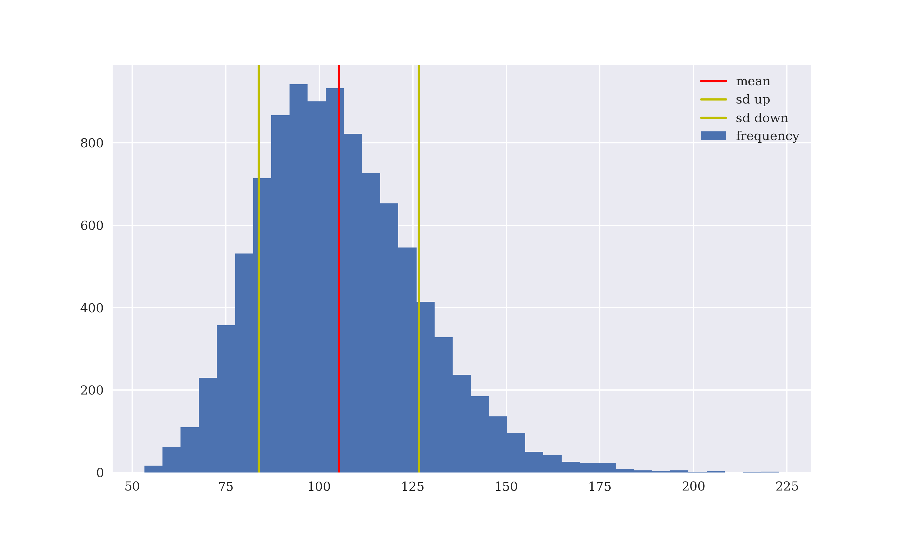
Figure 5-1. Simulated values for the stock price in Black-Scholes-Merton (1973)

Having the simulated stock price values available, makes European option pricing only a matter of two more vectorized operations.

In [70]: K = 105  

In [71]: CT = np.maximum(ST - K, 0)  

In [72]: CT[:8].round(1)
Out[72]: array([ 0. ,  5.4, 24.8,  0. , 20.4,  9.2,  2.7,  0. ])

In [73]: C0 = math.exp(-r * T) * CT.mean()  

In [74]: C0  
Out[74]: 8.120009539141193

The strike price of the option.

The payoff vector of the option.

The Monte Carlo estimator of the option price.

Completeness of Black-Scholes-Merton

What about the completeness of the Black-Scholes-Merton model economy ${ℰ}^{BSM}$? The previous section derives a Monte Carlo estimator for the (arbitrage) price of a European call option despite the fact that there are much more states of the economy $I\gg 2$ than financial assets traded $K=2$. Two observations can be made:

• General incompleteness: In a wider sense, the economy is incomplete because not every contingent claim can be replicated by a portfolio of the traded assets and because there is not a unique martingale measure (see 2FTAP).

• Specific completeness: In a narrow sense, the model is complete, because every contingent claim that can be represented as a function of the price vector of the stock $C_1=f\left(S_1^2\right)$ is replicable by positions in the bond and the stock.

When using Monte Carlo simulation to derive an estimator for the arbitrage price in the previous section, the fact is used that the model economy ${ℰ}^{BSM}$ is complete in the above specific sense. The payoff of the European call option only depends on the future price vector of the stock. What is missing so far is the replication portfolio and the resulting arbitrage price calculation to verify that the Monte Carlo simulation approach is justified.

The NumPy function used so far to solve replication problems np.linalg.solve requires a square (market payoff) matrix. In the Black-Scholes-Merton economy with only two traded financial assets and many more possible future states this prerequisite is not given. However, one can use a least-squares approach via np.linalg.lstsq to find a numerical solution to the replication problem.

In [75]: B0 = 100  

In [76]: M0 = np.array((B0, S0))  

In [77]: BT = B0 * np.ones(len(ST)) * math.exp(r * T)  

In [78]: BT[:4]  
Out[78]: array([105.12711, 105.12711, 105.12711, 105.12711])

In [79]: M = np.array((BT, ST)).T  

In [80]: M  
Out[80]: array([[105.12711,  72.61831],
                [105.12711, 110.35542],
                [105.12711, 129.77178],
                ...,
                [105.12711,  94.19527],
                [105.12711, 119.30886],
                [105.12711,  98.80359]])

In [81]: phi = np.linalg.lstsq(M, CT, rcond=None)[0]  

In [82]: phi  
Out[82]: array([-0.50337,  0.58428])

In [83]: np.mean((np.dot(M, phi) - CT))  
Out[83]: -3.425384420552291e-14

In [84]: np.dot(M0, phi)  
Out[84]: 8.090522690395254

The arbitrarily fixed price for the bond.

The price vector today for the two traded financial assets.

The future price vector of the bond given the initial price and the short rate.

The resulting market payoff matrix which is of rank 2 only — compared to 10,000 future states.

This solves the replication problem through least-squares representation. For the call option replication the bond is to be shorted (sold) and the stock is to be bought.

The average replication error, resulting, for example, from floating point inaccuracies and the numerical methods used, is not exactly zero but really close to it.

This calculates the arbitrage price given the (numerically) optimal replication portfolio. It is close to the Monte Carlo estimator from before.

Merton Jump-Diffusion Option Pricing

This section introduces another important model economy which dates back to Merton (1976) and adds a jump component to the stock price model of Black-Scholes-Merton (1973). The random jump component renders the model economy ${ℳ}^{M76}$ incomplete in general. However, in the discrete setting of this chapter one can apply the same numerical approaches for option pricing as introduced for ${ℰ}^{BSM}$ in the previous two sections. The model is called jump-diffusion model although a diffusion is only defined in a dynamic context.

In real financial time series, one observes jumps with some regularities. They might be caused by a stock market crash and by other rare and/or extreme events. The model by Merton (1976) allows to explicitly model such rare events and their impact on the price of financial instruments. Models without jumps are often not well suited to explain certain characteristics and phenomena as regularly observed in financial time series. The model is also capable of modeling both positive as well as negative jumps. While a negative jump (large drop) might be observed in practice for stock indices, positive jumps (spikes) occur in practice, for example, in volatility indices.

The Merton jump-diffusion economy ${ℰ}^{M76}$ is the same as the Black-Scholes-Merton economy ${ℰ}^{BSM}$ apart from the future price of the stock at time $T$ which can be simulated in this economy according to

with the $z_i^1,z_i^2$ being standard normally distributed and the $y_i$ being Poisson distributed with intensity $\lambda$ (see Jacod and Protter (2004), ch. 4). The jumps are log-normally distributed with expected value of $\mu$ and standard deviation of $\delta$ (see Jacod and Protter (2004), ch. 7). The expected jump size is:

To implement and simulate this model in Python requires the definition of additional parameters and the simulation of three random variables. Figure 5-2 shows the simulated values which can become negative given the parameters assumed and the Python code used.

In [85]: M0 = np.array((100, 100))   

In [86]: r = 0.05
         sigma = 0.2
         lmbda = 0.3
         mu = -0.3
         delta = 0.1
         rj = lmbda * (math.exp(mu + delta ** 2 / 2) - 1)
         T = 1.0
         I = 10000

In [87]: BT = M0[0] * np.ones(I) * math.exp(r * T)

In [88]: z = np.random.standard_normal((2, I))  
         z -= z.mean()  
         z /= z.std()  
         y = np.random.poisson(lmbda, I)  

In [89]: ST = S0 * (
             np.exp((r - rj - sigma ** 2 / 2) * T +
                    sigma * math.sqrt(T) * z[0]) +
             (np.exp(mu + delta * z[1]) - 1) * y
         )  

In [90]: ST.mean() * math.exp(-r * T)  
Out[90]: 100.63133302530244

In [91]: plt.figure(figsize=(10, 6))
         plt.hist(ST, bins=35, label='frequency');
         plt.axvline(ST.mean(), color='r', label='mean')
         plt.axvline(ST.mean() + ST.std(), color='y', label='sd up')
         plt.axvline(ST.mean() - ST.std(), color='y', label='sd down')
         plt.legend(loc=0);

Fixes the initial price vector of the two traded financial assets (bond and stock).

The first set of standard normally distributed random numbers.

The second set of standard normally distributed random numbers.

The set with Poisson distributed random numbers with intensity lambda.

The simulation of the stock price values at $T$ given the three sets of random numbers.

Calculates the discounted mean value of the simulated stock price.

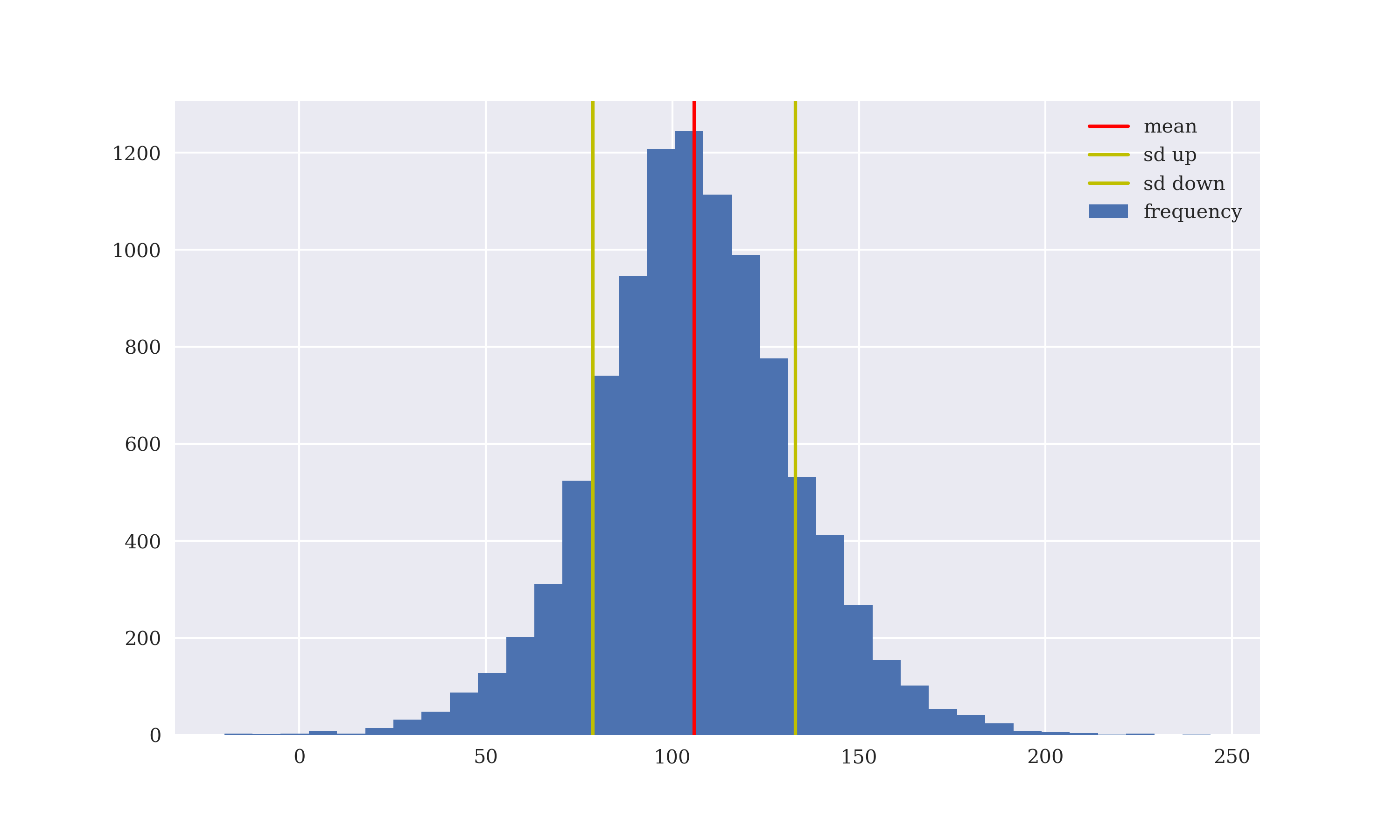
Figure 5-2. Simulated values for the stock price in Merton (1976)

Adding a maximum function to the stock price, Monte Carlo simulation avoids negative values (see Figure 5-3).

In [92]: ST = np.maximum(S0 * (
             np.exp((r - rj - sigma ** 2 / 2) * T +
                    sigma * math.sqrt(T) * z[0]) +
             (np.exp(mu + delta * z[1]) - 1) * y
         ), 0)  

In [93]: plt.figure(figsize=(10, 6))
         plt.hist(ST, bins=35, label='frequency')  
         plt.axvline(ST.mean(), color='r', label='mean')
         plt.axvline(ST.mean() + ST.std(), color='y', label='sd up')
         plt.axvline(ST.mean() - ST.std(), color='y', label='sd down')
         plt.legend(loc=0);

Maximum function …

… avoids negative values for the stock price.

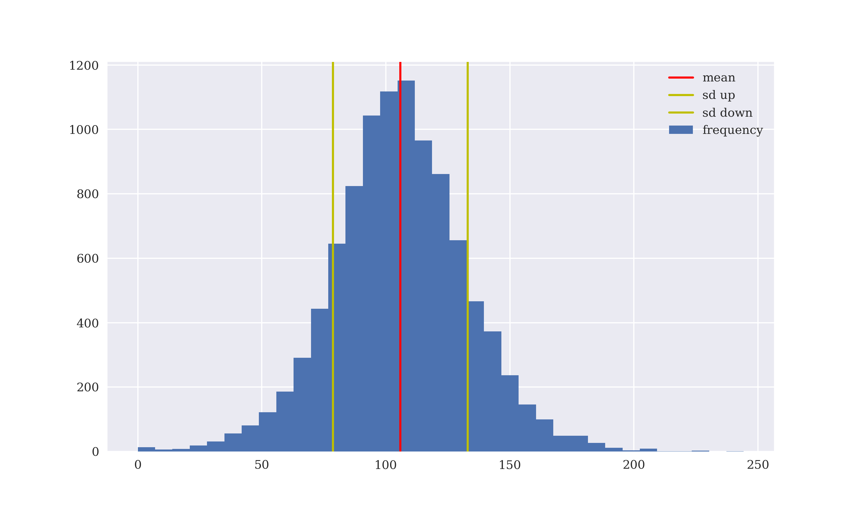
Figure 5-3. Simulated values (truncated) for the stock price in Merton (1976)

The final step is the pricing of the European call option through calculation of the Monte Carlo estimator and the approximate replication approach.

In [94]: K = 105

In [95]: CT = np.maximum(ST - K, 0)

In [96]: C0 = math.exp(-r * T)  * np.mean(CT)  

In [97]: C0  
Out[97]: 10.322864494488943

In [98]: M = np.array((BT, ST)).T

In [99]: phi = np.linalg.lstsq(M, CT, rcond=-1)[0]  

In [100]: phi  
Out[100]: array([-0.41918,  0.51909])

In [101]: np.mean(np.dot(M, phi) - CT)  
Out[101]: -2.5636381906224415e-14

In [102]: np.dot(M0, phi)  
Out[102]: 9.991506469652071