Chapter 1. Graph-Powered Machine Learning Methods
After completing this chapter, you should be able to:
-
List three basic ways that graph data and analytics can improve machine learning
-
Point out which graph algorithms have proved valuable for unsupervised learning
-
Extract graph features to enrich your training data for supervised machine learning
-
Describe how neural networks have been been extended to learn on graphs
-
Provide use cases and examples to illustrate graph-powered machine learning
-
Choose which types of graph-powered machine learning are right for you
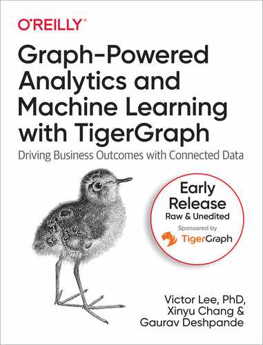
We now begin the third theme of our book: Learn. That is, we’re going to get serious about the core of machine learning: model training. Let’s review the machine learning pipeline that we introduced in Chapter 1. For convenience, we’ve shown it here again, as Figure 1-1. In the first part of this book, which explored the Connect theme. That theme fits the first two stages of the pipeline: data acquisition and data preparation. Graph databases make it easy to pull data from multiple sources into one connected database and to perform entity resolution.
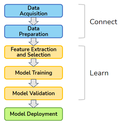
Figure 1-1. Machine learning pipeline
In this chapter, we’ll show how graphs enhance the central stages in the pipeline: feature extraction and all-important model training. Features are simply the characteristics or properties of your data entities, like the age of a person or the color of a sweater. Graphs offer a whole new realm of features which are based on how an entity connects to other entities. The addition of these unique graph-oriented features provides machine learning with better raw materials with which to build its models.
This chapter has four sections. The first three sections each describe a different way that graphs enhance machine learning. First, we will start with unsupervised learning, as it is similar to the techniques we discussed in the Analyze section of the book. Second, we will turn to graph feature extraction for supervised and unsupervised machine learning. Third, we culminate with model training directly on graphs, for both supervised and unsupervised approaches. This includes techniques for clustering, embedding, and neural networks. Because they work directly on graphs, some graph databases are now available to offer in-database machine learning. The fourth section reviews the various methods in order to compare them and to help you decide which approaches will meet your needs.
Unsupervised Learning with Graph Algorithms
Unsupervised learning is the forgotten sibling of supervised learning and reinforcement learning, who together form the three major branches of machine learning. If you want your AI system to learn how to do a task, to classify things according to your categories, or to make predictions, you want to use supervised learning and/or reinforcement learning. Unsupervised learning, however, has the great advantage of being self-sufficient and ready-to-go. Unlike supervised learning, you don’t need to already know the right answer for some cases. Unlike reinforcement learning, you don’t have to be patient and forgiving as you stumble through learning by public trial and error. Unsupervised learning simply takes the data you have and reports what it learned
Think of each unsupervised learning technique as a specialist who is confident in their own ability and specialty. We call in the specialist, they tell us something that we hadn’t noticed before, and we thank them for their contribution. An unsupervised learning algorithm can look at your network of customers and sales and tell you what are your actual market segments, which may not fit simple ideas of age and income. An unsupervised learning algorithm can point out customer behavior that is an outlier, far from normal, by determining “normal” from your data, not from your preconceptions. For example, an outlier can point out which customers are likely to churn (choose a competitor’s product or service).
The first way we will learn from graph data is by applying graph algorithms to discover patterns or characteristics of our data. Earlier in the book, in the Analyze section, we took our first detailed look at graph algorithms. We’ll now look at additional families of graph algorithms which go deeper. The line between Analyze and Learn can be fuzzy. What characterizes these new algorithms is that they look for or deal with patterns. They could all be classified as pattern discovery or data mining algorithms for graphs.
Finding Communities
When people are allowed to form their own social bonds, they will naturally divide into groups. No doubt you observed this, in school, in work, in recreation, and in online social networks. We form or join communities. However, graphs can depict any type of relationship, so it can be valuable to know about other types of communities in your data. Use cases include:
-
Finding a set of highly interconnected transactions among a set of parties / institutions / locations / computer networks which are out of the ordinary: is this a possible financial crime?
-
Finding pieces of software / regulation / infrastructure which are highly connected and interdependent. It is good that they are connected, as a sign of popularity, value, and synergy? Or it is a concerning sign that some components are unable to stand on their own as expected?
-
In the sciences (ecology, cell biology, chemistry), finding a set of highly interacting species / proteins is evidence of (inter)dependence and can suggest explanations for such dependence.
Community detection can be used in connection with other algorithms. For example, first use a PageRank or centrality algorithm to find an entity of interest (e.g., a known or suspected criminal). Then find the community to which they belong. You could also swap the order. Find communities first, then count how many parties of note are within that community. Again, whether that is healthy or not depends on the context. Algorithms are your tools, but you are the craftsperson.
What is a Community?
In network science, a community is a set of vertices that have a higher density of connections within the group than to outside the group. Specifically, we look at the edge density of the community, which is the number of edges between members divided by the number of vertices. A significant change in edge density provides a natural boundary between who is in and who is not. Network scientists have defined several different classes of communities based on how densely they are interconnected. Higher edge density implies a more resilient community.
The following three types of communities span the range from weakest density to strongest density and everything in between.
- Connected Component
-
You are in if you have a direct connection to one or more members of the community. Requiring only one connection, this is the weakest possible density. In graph theory, if you simply say “component,” it refers to a connected community plus the edges that connect them.
- K-Core
-
You are in if you have a direct connection to k or more members of the community, where k is a positive integer.
- Clique
-
You are in if you have a direct connection to every other member of the community. This is the strongest possible density. Note that clique has a specific meaning in network science and graph theory.
Note
A connected component is a k-core where k = 1. A clique containing c vertices is a k-core where k = (c -1), the largest possible value for k.
Figure 1-2 illustrates examples of these three definitions of community. On the left, there are three separate connected components, represented by the three different shadings. In the center, there are two separate k-cores for k = 2. The lower community, the rectangle with diagonal connections, would also satisfy k = 3 because each member vertex connects to three others. On the right, there are two separate cliques.
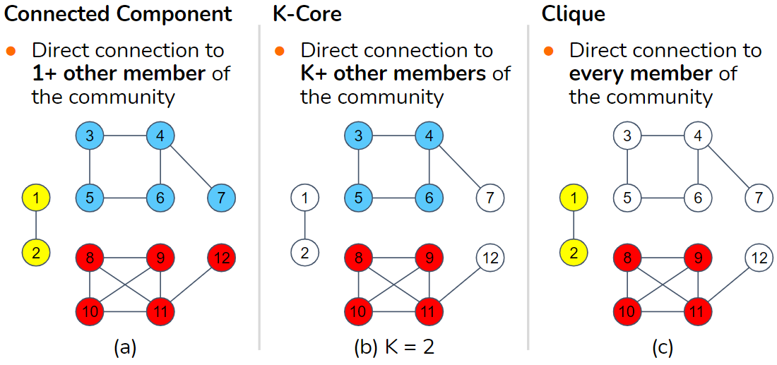
Figure 1-2. Three definitions of community, from weakest at left to strongest at right
Modularity-Based Communities
In many applications, however, we don’t have a specific value of k in mind. In the spirit of unsupervised learning, we want the data itself to tell us what is dense enough. To address this, network scientists came up with a measure called modularity which looks at relative density, comparing the density within communities versus the density of connections between communities. This is like looking at the density of streets within cities versus the road density between cities. Now imagine the city boundaries are unknown; you just see the roads. If you propose a set of city boundaries, modularity will rate how good a job you did of maximizing the goal of “dense inside; not dense outside.” Modularity is a scoring system, not an algorithm. A modularity-based community algorithm finds the community boundaries which produce the highest modularity score.
The Louvain algorithm, named after the University of Louvain, is perhaps the fastest algorithm for finding community boundaries with a very high modularity. It works hierarchically by forming small local communities, then substituting each community with a single meta-vertex, and repeating by forming local communities of meta-vertices.
To measure modularity (Q), we first partition the vertices into a set of communities so that every vertex belongs to one community. Then, considering each edge as one case, we calculate some totals and averages:
Q
=[
actual fraction of edges that fall within a community]
minus [expected fraction of edges if edges were distributed at random]
“Expected” is used in the statistical sense: If you flip a coin many times, you expect 50/50 odds of heads vs. tails. Modularity can handle weighted edges by using weights instead of simple counts:
Q = [average weight of edges that fall within a community]
minus [expected weight of edges if edges were distributed at random]
Note that the average is taken over the total number of edges. Edges which run from one community to another add zero to the numerator and add their weight to the denominator. It is designed this way so that edges which run between communities hurt your average and lower your modularity score.
What do we mean by “distributed at random”? Each vertex v has a certain number of edges which connect to it: the degree of a vertex is d(v) = total number (or total weight) of v’s edges. Imagine that each of these d(v) edges picks a random destination vertex. The bigger d(v) is, the more likely that one or more of those random edges will make a connection to a particular destination vertex. The expected (i.e., statistical average) number of connections between a vertex v1 and a vertex v2 can be computed with Equation 1-1.
Equation 1-1. Expected number of connections between two vertices based on their degrees
where m is the total number of edges in the graph. For the mathematically inclined, the complete formula is shown in Equation 1-2 below, where wt(i,j) is the weight of the edge between i and j, com(i) is the community ID of vertex i, and δ(a,b) is the Kronecker delta function which equals 1 if a and b are equal, 0 otherwise.
Equation 1-2. Definition of modularity
Finding Similar Things
Being in the same community is not necessarily an indicator of similarity. For example, a fraud ring is a community, but it requires different persons to play different roles. Moreover, one community can be composed of different types of entities. For example, a grassroots community centered around a sports team could include persons, businesses selling fan paraphernalia, gathering events, blog posts, etc. If you want to know which entities are similar, you need a different algorithm. Fans who attend the same events and buy the same paraphernalia intuitively seem similar; to be sure, we need a well-defined way of assessing similarity.
Efficient and accurate measurement of similarity is one of the most important tools for businesses because it is what underlies personalized recommendation. We have all seen recommendations from Amazon or other online vendors suggest that we consider a product because “other persons like you bought this.” If the vendor’s idea of “like you” is too broad, they may make some silly recommendations which annoy you. They want to use several characteristics they know or infer about you and your interests to filter down the possibilities, and then see what similar customers did. Similarity is used not only for recommendations but also for following up after detecting a situation of special concern, such as a security vulnerability or a crime of some sort. We found this case. Are there similar cases out there?
Simply finding similar things does not necessarily qualify as machine learning. The first two types of similarity we will look at are important to know, but they aren’t really machine learning. These types are graph-based similarity and neighborhood similarity. They lead to the third type, role similarity, which can be considered unsupervised machine learning. Role similarity looks deeply and iteratively in the graph to refine its understanding of the graph’s structural patterns.
Similarity values are a prerequisite for at least three other machine learning tasks, clustering, classification, and link prediction. Clustering is putting things that are close together into the same group. “Close” does not necessarily mean physically close together; it means…similar. People often confuse communities with clusters. Communities are based on density of connections; clusters are based on similarity of the entities. Classification is deciding which of several predefined categories an item should be placed into. A common meta-approach is to say that an item should be put in the same category as that of similar items which have a known category. If things that look like and walk like it are ducks, then we conclude that it is a duck. Link prediction is making a calculated guess that a relationship, which does not currently exist in the dataset, either does exist or will exist in the real world. In many scenarios, entities which have similar neighborhoods (circumstances) are likely to have similar relationships. The relationship could be anything: a person-person relationship, a financial transaction, or a job change. Investigators, actuaries, gamblers, and marketers all seek to do accurate link prediction. As we can see, similarity pops up as a prerequisite for numerous machine learning tasks.
Graph-Based Similarity
What makes two things similar? We usually identify similarities by looking at observable or known properties: color, size, function, etc. A passenger car and a motorcycle are similar because they are both motorized vehicles for one or a few passengers. A motorcycle and a bicycle are similar because they are both two-wheeled vehicles. But, how do we decide whether a motorcycle is more similar to a car or to a bicycle? For that matter, how would we make such decisions for a set of persons, products, medical conditions, or financial transactions? We need to agree upon a system for measuring similarity. But, to take an unsupervised approach, is there some way that we can let the graph itself suggest how to measure similarity?
A graph can give us contextual information to help us decide how to determine similarity. Consider the axiom
A vertex is characterized by its properties, its relationships, and its neighborhood.
Therefore, if two vertices have similar properties, similar relationships, and similar neighborhoods, then they should be similar. What do we mean by similar neighborhoods? Let’s start with a simpler case: the exact same neighborhood.
Two entities are similar if they connect to the same neighbors.
In Figure 1-3, Person A and Person B have three identical types of edges (purchased, hasAccount, and knows), connecting to the three exact same vertices (Phone model Y, Bank Z, and Person C, respectively). It is not necessary, however, to include all types of relationships or to give them equal weight. If you care about social networks, for example, you can consider only friends. If you care about financial matters, you can consider only financial relationships.
Figure 1-3. Two persons sharing the same neighborhood
To reiterate the difference between community and similarity: All five entities in Figure 1-3 are part of a connected component community. However, we would not say that all five are similar to one another. The only case of similarity suggested by these relationships is Person A being similar to Person B.
Neighborhood Similarity
It’s rare to find two entities which have exactly the same neighborhoods. We’d like a way to measure and rank the degree of neighborhood similarity. The two most common measures for ranking neighborhood similarity are Jaccard similarity and cosine similarity.
Jaccard Similarity
Jaccard similarity measures the relative overlap between two general sets. Suppose you run Bucket List Travel Advisors, and you want to compare your most frequent travelers to one another based on which destinations they have visited. Jaccard similarity would be a good method for you to use; the two sets would be the destinations visited by each of two customers being compared. To formulate Jaccard similarity in general terms, suppose the two sets are N(a), the neighborhood of vertex a, and N(b), the neighborhood of vertex b. Equation 1-3 gives a precise definition of neighborhood-based Jaccard similarity:
Equation 1-3. Jaccard neighborhood similarity
The maximum possible score is 1, which occurs if a and b have exactly the same neighbors. The minimum score is 0, if they have no neighbors in common.
Consider the following example. Three travelers, A, B, and C, have traveled to the following places as shown in Table 1-1.1
| Bucket List’s Top 10 | A | B | C |
| Amazon Rainforest, Brazil | ✔ | ✔ | |
| Grand Canyon, USA | ✔ | ✔ | ✔ |
| Great Wall, China | ✔ | ✔ | |
| Machu Picchu, Peru | ✔ | ✔ | |
| Paris, France | ✔ | ✔ | |
| Pyramids, Egypt | ✔ | ||
| Safari, Kenya | ✔ | ||
| Taj Mahal, India | ✔ | ||
| Uluru, Australia | ✔ | ||
| Venice, Italy | ✔ | ✔ |
Using the table’s data, the Jaccard similarities for each pair of travelers can be computed.
-
A and B have three destinations in common (Amazon, Grand Canyon, Machu Picchu). Collectively they have been to nine destinations. jaccard(A, B) = 3/9 = 0.33.
-
B and C have only one destination in common (Grand Canyon). Collectively they have been to ten destinations. jaccard(B, C) = 1/10 = 0.10.
-
A and C have three destinations in common (Grand Canyon, Paris, Venice). Collectively they have been to seven destinations. jaccard(A, C) = 3/7 = 0.43.
Among these three, A and C are the most similar. As the proprietor, you might suggest that C visit some of the places that A has visited, such as the Amazon and Machu Picchu. Or you might try to arrange a group tour, inviting both of them to somewhere they both have not been to, such as Uluru, Australia.
Cosine Similarity
Cosine similarity measures the alignment of two sequences of numerical characteristics. The name comes from the geometric interpretation in which the numerical sequence is the entity’s coordinates in space. The data points on the grid (the other type of “graph”) in Figure 1-4 illustrate this interpretation.

Figure 1-4. Geometric interpretation of numeric data vectors.
Point A represents an entity whose feature vector is (2,0). B’s feature vector is (3,1). Now we see why we call a list of property values a “vector.” The vectors for A and B are somewhat aligned. The cosine of the angle between them is their similarity score. If two vectors are pointed in exactly the same direction, the angle between them is 0; the cosine of their angle is 1. cos(A,C) is 0 because A and C are perpendicular; the vectors (2,0) and (0,2) have nothing in common. cos(A,D) is -1 because A and D are pointed in opposite directions. So, cos(x,y) = 1 for two perfectly similar entities, 0 for two perfectly unrelated entities, and -1 for two perfectly anticorrelated entities.
Suppose you have scores across several categories or attributes for a set of entities. You want to cluster the entities, so you need an overall similarity score between entities. The scores could be ratings of individual features of products, employees, accounts, etc. Let’s continue the example of Bucket List Travel Advisors. This time, each customer has rated their enjoyment of a destination on a scale of 1 to 10, so we have numerical values, not just yes/no.
| Bucket List’s Top 10 | A | B | C |
| Amazon Rainforest, Brazil | 8 | ||
| Grand Canyon, USA | 10 | 6 | 8 |
| Great Wall, China | 5 | 8 | |
| Machu Picchu, Peru | 8 | 7 | |
| Paris, France | 9 | 4 | |
| Pyramids, Egypt | 7 | ||
| Safari, Kenya | 10 | ||
| Taj Mahal, India | 10 | ||
| Uluru, Australia | 9 | ||
| Venice, Italy | 7 | 10 |
Here are steps for using this table to compute cosine similarity between pairs of travelers.
-
List all the possible neighbors and define a standard order for the list so we can form vectors. We will use the top-down order in Table 10-1, from Amazon to Venice.
-
If the graph has D possible neighbors, this gives each vertex a vector of length D. For Table 10-2, D = 10. Each element in the vector is either the edge weight, if that vertex is a neighbor, or the null score if it isn’t a neighbor.
-
Determining the right null score is important so that your similarity scores mean what you want them to mean. If a 0 means someone absolutely hated a destination, it is wrong to assign a 0 if someone has not visited a destination. A better approach is to normalize the scores. You can either normalize by entity (traveler), by neighbor/feature (destination), or by both. The idea is to replace the empty cells with a default score. You could set the default to be the average destination, or you could set it a little lower than that, because not having visited a place is a weak vote against that place. For simplicity, we won’t normalize the scores; we’ll just use 6 as the default rating. Then traveler A’s vector is Wt(A) = [8, 10, 5, 8, 9, 6, 6, 6, 6, 7].
-
Then, apply the formula in Equation 1-4 for cosine similarity:
Equation 1-4. Cosine neighborhood similarity
Wt(a) and Wt(b) are the neighbor connection weight vectors for a and b, respectively. The numerator goes element by element in the vectors, multiplying the weight from a by the weight from b, then adding together these products. The more that the weights align, the larger the sum we get. The denominator is a scaling factor, the Euclidean length of vector Wt(a) multiplied by the length of vector Wt(b).
Let’s look at one more use case, people who rate movies, to compare how Jaccard and cosine similarity work. In Figure 1-5, we have two persons A and B who have each rated three movies. They have both rated two of the same movies, Black Panther and Frozen.

Figure 1-5. Similarity of persons who rate movies
If we only care about what movies the persons have seen and not about the scores, then Jaccard similarity is sufficient and easier to compute. This would also be your choice if scores were not available or if the relationships were not numeric. The Jaccard similarity is (size of overlap) / (size of total set) = 2 / 4 = 0.5. That seems like a middling score, but if there are hundreds or thousands of possible movies they could have seen, then it’s a very high score.
If we want to take the movie ratings into account to see how similar are A’s and B’s taste, we should use cosine similarity. Assuming the null score is 0, then A’s neighbor score vector is [5, 4, 3, 0] and B’s is [4, 0, 5, 5]. For cosine similarity, the numerator is [5, 4, 3, 0] ⋅ [4, 0, 5, 5] = (5)(4)+(4)(0)+(3)(5)+(0)(5) = 35. The denominator =
Tip
Use Jaccard similarity when the features of interest are yes/no or categorical variables.
Use cosine similarity when you have numerical variables. If you have both types, you can use cosine similarity and treat your yes/no variables as having values 1/0
Role Similarity
Earlier we said that if two vertices have similar properties, similar relationships, and similar neighborhoods, then they should be similar. We first examined the situation in which the neighborhoods contained some of the exact same members, but let’s look at the more general scenario in which the individual neighbors aren’t the same, just similar.
Consider a graph of family relationships. One person, Jordan, has two living parents, is married to someone who was born in a different country, and they have three children together. Another person, Kim, also has two living parents, is married to someone born in another country, and together they have four children. None of the neighboring entities (parents, spouses, children) are the same. The number of children is similar but not exactly the same. Nevertheless, Jordan and Kim are similar because they have similar relationships. This is called role similarity.
Moreover, if Jordan’s spouse and Kim’s spouse are similar, that’s even better. If Jordan’s children and Kim’s children are similar in some way (ages, hobbies, etc.), that’s even better. You get the idea. Instead of people, these could be products, components in a supply chain or power distribution network, or financial transactions.
Two entities have similar roles if they have similar relationships to entities which themselves have similar roles.
This is a recursive definition: A and B are similar if their neighbors are similar. Where does it stop? What is the base case where we can say for certain how much two things are similar?
SimRank
In their 2002 paper, Glen Jeh and Jennifer Widom proposed SimRank which measures similarity by having equal length paths from A and B both reach the same individual; e.g., if Jordan and Kim share a grandparent, that contributes to their SimRank score. The formal definition is shown in Equation 1-5 below.
Equation 1-5. SimRank
In(a) and In(b) are the sets of in-neighbors of vertices a and b, respectively, u is a member of In(a), v is a member of In(b), and C is a constant between 0 and 1 to control the rate at which neighbors’ influence decreases as distance from a source vertex increases. Lower values of C mean a more rapid decrease. SimRank computes a N × N array of similarity scores, one for each possible pair. This differs from cosine and Jaccard similarity which compute a single pair’s score on demand. It is necessary to compute the full array of SimRank scores because the value of SimRank(a,b) depends of the SimRank score of pairs of their neighbors (e.g., SimRank(u,v)), which in turn depends on their neighbors, and so on. To compute SimRank, you initialize the array so that SimRank(a,b) = 1 if a = b; otherwise it is 0. Then calculate a revised set of scores by applying Equation 1-5 for each pair (a,b) where the SimRank scores on the right side are from the previous iteration. Note that this is like PageRank’s computation except that we have N × N scores instead of just N scores. SimRank’s reliance on eventually reaching a shared individual, and through equal length paths, is too rigid for some cases. SimRank does not fully embrace the idea of role similarity. Two individuals in two completely separate graphs, e.g. graphs representing two unrelated families or companies, should be able to show role similarity.
RoleSim
To address this shortcoming, Ruoming Jin et al.2 introduced RoleSim in 2011. RoleSim starts with the (over)estimate that the similarity between any two entities is the ratio of the sizes of their neighbors. The initial estimate for RoleSim(Jordan, Kim) would be 5/6. RoleSim then uses the current estimated similarity of your neighbors to make an improved guess for the next round. Equation 1-6 has the formal definition of RoleSim.
Equation 1-6. RoleSim
The parameter ? is similar to SimRank’s C. The main difference is the function M. M(a,b) is a bipartite matching between the neighborhoods of a and b. This is like trying to pair up the three children of Jordan with the four children of Kim. M(Jordan, Kim) will consist of three pairs (and one child left out). Moreover, there are 24 possible matchings. For computational purposes (not actual social dynamics), assume that the oldest child of Jordan selects a child of Kim; there are four options. The next child of Jordan picks from the three remaining children of Kim, and the third child of Jordan can choose from the two remaining children of Kim. This yields (4)(3)(2) = 24 possibilities. The max term in the equation means that we select the matching that yields the highest sum of RoleSim scores for the three chosen pairs. If you think of RoleSim as a compatibility score, then we are looking for the combination of pairings that gives us the highest total compatibility of partners. You can see that this is more computational work than SimRank, but the resulting scores have nicer properties:
-
There is no requirement that the neighborhoods of a and b every meet.
-
If the neighborhoods of a and b “look” exactly the same, because they have the same size, and each of the neighbors can be paired up so that their neighborhoods look the same, and so on, then their RoleSim score will be a perfect 1. Mathematically, this level of similarity is called automorphic equivalence.
This idea of looking at neighbors of neighbors to get a deeper sense of similarity will come up again later in the chapter.
Finding Frequent Patterns
As we’ve said early on in this book, graphs are wonderful because they make it easy to discover and analyze multi-connection patterns based on connections. In the Analyze section of the book, we talked about finding particular patterns, and we will return to that topic later in this chapter. In the context of unsupervised learning, the goal is to:
Find any and all patterns which occur frequently.
Computer scientists call this the Frequent Subgraph Mining task, because a pattern of connections is just a subgraph. This task is particularly useful for understanding natural behavior and structure, such as consumer behavior, social structures, biological structures, and even software code structure. However, it also presents a much more difficult problem. “Any and all” patterns in a large graph means a vast number of possible occurrences to check. The saving grace is the threshold parameter T. To be considered frequent, a pattern must occur at least T times. If T is big enough, that could rule out a lot of options early on. The example below will show how T is used to rule out small patterns so that they don’t need to be considered as building blocks for more complex patterns.
There any many advanced approaches to try to speed up frequent subgraph mining, but the basic approach is to start with 1-edge patterns, keep the patterns that occur at least T times, and then try to connect those patterns to make bigger patterns:
-
Group all the edges according to their type and the types of their endpoint vertices. For example, Shopper-(bought)-Product is a pattern.
-
Count how many times each pattern occurs.
-
Keep all the frequent patterns (having at least T members) and discard the rest.
For example, we keep Shopper-(lives_in)-Florida but eliminate Shopper-(lives_in)-Guam because it is infrequent. -
Consider every pair of groups that have compatible vertex types (e.g., groups 1 and 2 both have a Shopper vertex), and see how many individual vertices in group 1 are also in group 2. Merge these individual small patterns to make a new group for the larger pattern. For example, we merge the cases where the same person in the frequent pattern Shopper-(bought)-Blender was also in the frequent pattern Shopper-(lives_in)-Florida.
-
Repeat steps 2 and 3 (filtering for frequency) for these newly formed larger patterns.
-
Repeat step 4 using the expanded collection of patterns.
-
Stop when no new frequent patterns have been built.
There is a complication with counting (step 2). The complication is isomorphism, how the same set of vertices and edges can fit a template pattern in more than one way. Consider the pattern A-(friend_of)-B. If Jordan is a friend of Kim, which implies that Kim is a friend of Jordan, is that one instance of the pattern or two? Now suppose the pattern is “find pairs of friends A and B who are both friends with a third person C.” This forms a triangle. Let’s say Jordan, Kim, and Logan form a friendship triangle. There are six possible ways we could assign Jordan, Kim, and Logan to the variables A, B, and C. You need to decide up front whether these types of symmetrical patterns should be counted separately or merged into one instance, and then make sure your counting method is correct.
Summary
Graph algorithms can perform unsupervised machine learning on graph data. Key takeaways from this section are as follows:
-
Community detection algorithms find densely interconnected sets of entities.
-
Neighborhood similarity algorithms find entities who have similar relationships to others.
-
Clustering is grouping by nearness, and similarity is proxy for physical nearness.
-
Link prediction uses clues such as neighborhood similarity to predict whether an edge is likely to exist between two vertices.
-
Frequent pattern mining algorithms find patterns of connections which occur frequently.
Extracting Graph Features
In the previous section, we showed how you can use graph algorithms to perform unsupervised machine learning. In most of those examples, we analyzed the graph as a whole to discover some characteristics, such as communities or frequent patterns.
In this section, you’ll learn how graphs can provide additional and valuable features to describe and help you understand your data. A graph feature is a characteristic that is based on the pattern of connections in the graph. A feature can either be local – attributed to the neighborhood of an individual vertex or edge – or global – pertaining to the whole graph or a subgraph. In most cases, we are interested in vertex features – characteristics of the neighborhood around a vertex. That’s because vertices usually represent the real world entities which we want to model with machine learning.
When an entity (an instance of a real-world thing) has several features and we arrange those features in a standard order, we call the ordered list a feature vector. Some of the methods we’ll look at in this section provide individual features; others produce entire sets of features. You can concatenate a vertex’s entity properties (the ones that aren’t based on connections) with its graph features obtained from one or more of the methods discussed here to make a longer, richer feature vector. We’ll also look at a special self-contained feature vector called an embedding that summarizes a vertex’s entire neighborhood.
These features can provide insight as is, but one of their most powerful uses is to enrich the training data for supervised machine learning. Feature extraction is one of the key phases in a machine learning pipeline (refer back to Figure 1-1). For graphs, this is particularly important because traditional machine learning techniques are designed for vectors, not for graphs. So, in a machine learning pipeline, feature extraction is also where we transform the graph into a different representation.
In the sections that follow, we’ll look at three key topics: domain-independent features, domain-dependent features, and the exciting developments in graph embedding.
Domain-Independent Features
If graph features are new to you, the best way to understand them is to look at simple examples that would work for any graph. Because these features can be used regardless of the type of data we are modeling, we say they are domain-independent. Consider the graph in Figure 1-6. We see a network of friendships, and we count occurrences of some simple domain-independent graph features.
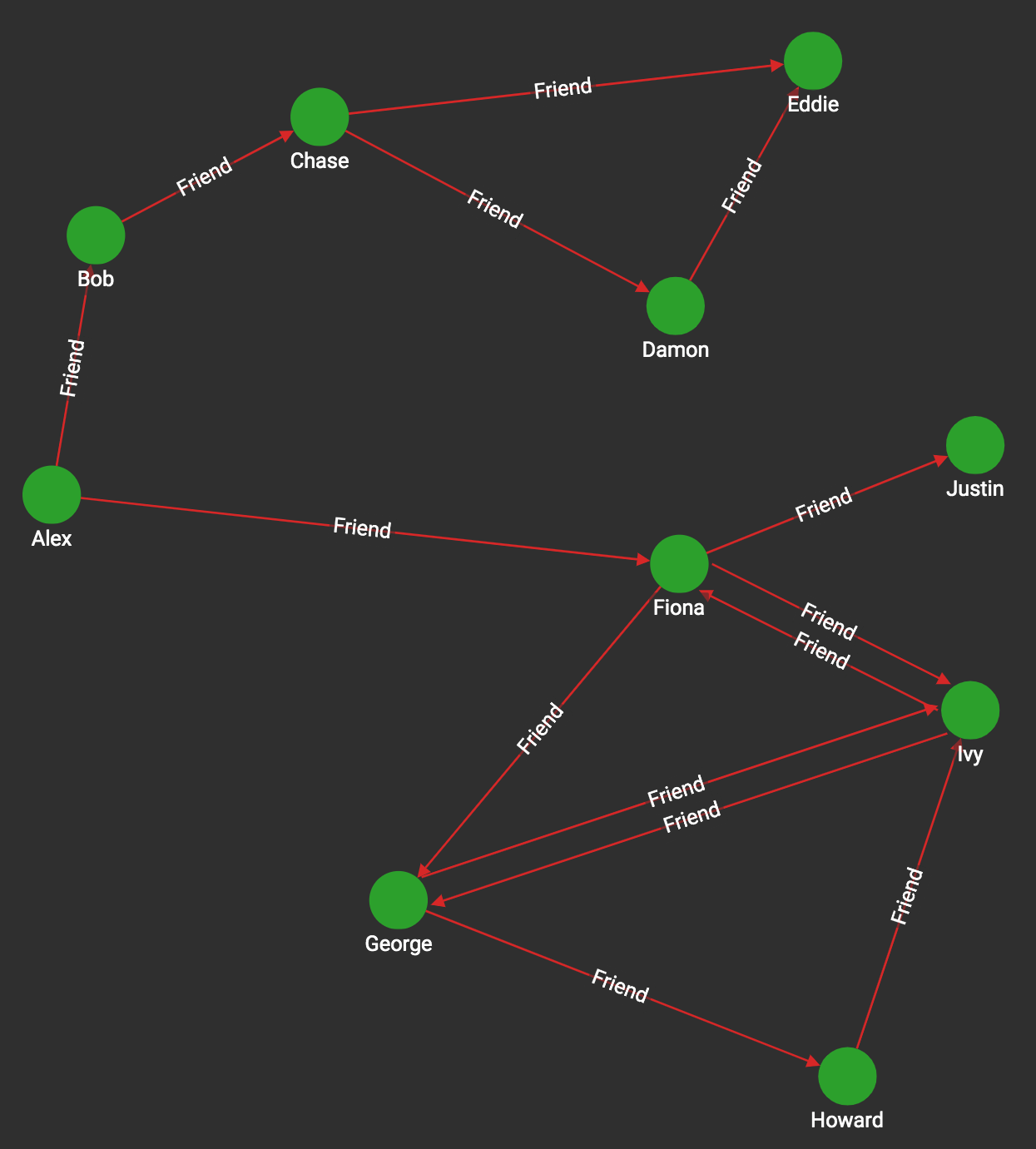
Figure 1-6. Graph with directed friendship edges
Table 1-3 shows the results for four selected vertices (Alex, Chase, Fiona, Justin) and four selected features.
| Number of in-neighbors | Number of out-neighbors | Number of vertices within 2 forward hops | Number of triangles (ignoring direction) | |
| Alex | 0 | 2 (Bob, Fiona) | 6 (B, C, F, G, I, J) | 0 |
| Chase | 1 (Bob) | 2 (Damon, Eddie) | 2 (D, E) | 1 (Chase, Damon, Eddie) |
| Fiona | 2 (Alex, Ivy) | 3 (George, Ivy, Justin) | 4 (G, I, J, H) | 1 (Fiona, George, Ivy) |
| Justin | 1 (Fiona) | 0 | 0 | 0 |
You could easily come up with more features, by looking farther than one or two hops3, by considering generic weight properties of the vertices or edges, and by calculating in more sophisticated ways: computing average, maximum, or other functions. Because these are domain-independent features, we are not thinking about the meaning of “person” or “friend”. We could change the object types to “computers” and “sends data to”. Domain-independent features, however, may not be the right choice for you if there are many types of edges with very different meanings.
Graphlets
Another option for extracting domain-independent features is to use graphlets4. Graphlets are small subgraph patterns, which have been systematically defined so that they include every possible configuration up to a given size limit. Figure 1-7 shows all 72 graphlets for subgraphs up to five vertices (or nodes). Note that the figure shows two types of identifiers: shape IDs (G0, G1, G2, etc.) and graphlet IDs (1, 2, 3, etc.). Shape G1 encompasses two different graphlets: graphlet 1, when the reference vertex is on the end of the 3-vertex chain, and graphlet 2, when the reference vertex is in the middle.
Counting the occurrences of every graphlet pattern around a given vertex provides a standardized feature vector which can be compared to any other vertex in any graph. This universal signature lets you cluster and classify entities based on their neighborhood structure, for applications such as predicting the world trade dynamics of a nation5 or link prediction in dynamic social networks like Facebook.6
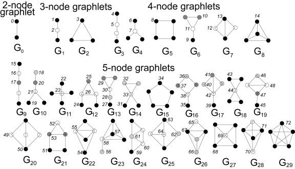
Figure 1-7. Graphlets up to five vertices (or nodes) in size7
A key rule for graphlets is that they are the induced subgraph for a set of vertices within a graph of interest. Induced means that they include ALL the edges that the base graph has among the selected set of vertices. This rule causes each particular set of vertices to match at most one graphlet pattern. For example, consider the four persons Fiona, George, Howard, and Ivy in Figure 1-6. Which shape and graphlet do they match, if any? It’s shape G7, because those four persons form a rectangle with one cross connection. They do not match shape G5, the square because of that cross connection between George and Ivy. While we’re talking about that cross connection, look carefully at the two graphlets for shape G7, graphlets 12 and 13. Graphlet 13’s source node is located at one end of the cross connection, just as George and Ivy are. This means graphlet 13 is one of their graphlets. Fiona and Howard are at the other corners of the square, which don’t have the cross connection. Therefore they have graphlet 12 in their graphlet portfolios.
There is obviously some overlap between the ad hoc features we first talked about (e.g., number of neighbors) and graphlets. Suppose a vertex A has three neighbors B, C, and D, as shown in Figure 1-8. However, we do not know about any other connections. What do we know about its graphlets?
-
It exhibits the graphlet 0 pattern three times. Counting the occurrences is important.
-
Now consider subgraphs with three vertices.We can define three different subgraphs containing A: (A, B, C), (A, B, D), and (A, C, D). Each of those threesomes satisfies either graphlet 2 or 3. Without knowing about the connections among B, C, and D (the dotted-line edges in the figure), we can be more specific.
-
Considering all four vertices, we might be tempted to say they match graphlet 7. Since there might be other connections between B, C, and D, it might actually be a different graphlet. Which one? Graphet 11 if there’s one peripheral connection, graphlet 13 if it’s two connections, or graphlet 14 if it’s all three possible connections.
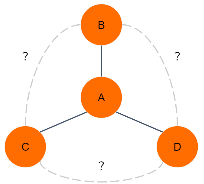
Figure 1-8. Immediate neighbors and graphlet implications
The advantage of graphlets is that they are thorough and methodical. Checking for all graphlets up to 5-node size is equal to considering all the details of the source vertex’s 4-hop neighborhood. You could run an automated graphlet counter without spending time and money to design custom feature extraction. The disadvantage of graphlets is that they can require a lot of computational work, and it might be more productive to focus on a more selective set of domain-dependent features. We’ll cover these types of features shortly.
Graph Algorithms
Here’s a third option for extracting domain-independent graph features: graph algorithms! In particular, the centrality and ranking algorithms which we discussed in the Analyze section of the book work well because they systematically look at everything around a vertex and produce a score for each vertex. Figures 10-9 and 10-10 show the PageRank and closeness centrality8 scores respectively for the graph presented earlier in Figure 1-7. For example, Alex has a PageRank score of 0.15 while Eddie has a PageRank score of 1. This tells us that Eddie is valued by his peers much more than Alex. Eddie’s ranking is due not only to the number of connections, but also to the direction of edges. Howard, who like Eddie has two connections and is at the far end of the rough “C” shape of the graph, has a PageRank score of only 0.49983 because one edge comes in and the other goes out.
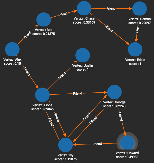
Figure 1-9. PageRank scores for the friendship graph.
The closeness centrality scores in Figure 1-10 tell a completely different story. Alex has a top score of 0.47368 because she is at the middle of the C. Eddie and Howard have scores at or near the bottom, 0.2815 and 0.29032 respectively, because they are at the ends of the C.
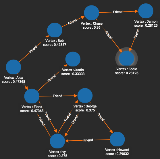
Figure 1-10. Closeness centrality scores for the friendship graph
The main advantage of domain-Independent feature extraction is its universality: generic extraction tools can be designed and optimized in advance, and the tools can be applied immediately on any data. Its unguided approach, however, can make it a blunt instrument.
Domain-independent feature extraction has two main drawbacks. Because it doesn’t pay attention to what type of edges and vertices it considers, it can group together occurrences that have the same shape but have radically different meanings. The second drawback is that it can waste resources computing and cataloging features which have no real importance or no logical meaning. Depending on your use case, you may want to focus on a more selective set of domain-dependent features.
Domain-Dependent Features
A little bit of domain knowledge can go a long way towards making your feature extraction smarter and more efficient.
When extracting domain-dependent features, the first thing you want to do is pay attention to the vertex types and edge types in your graph. It’s helpful to look at a display of your graph’s schema. Some schemas break down information hierarchically into graph paths, such as City-(IN)-State-(IN)-Country or Day-(IN)-Month-(IN)-Year. This is a graph-oriented way of indexing and pre-grouping data according to location or date. This is the case in a graph model for South Korean COVID-19 contact tracing data, shown in Figure 1-11. While City-to-County and Day-to-Year are each 2-hop paths, those paths are simply baseline information and do not hold the significance of a 2-hop path like Patient-(INFECTED_BY)-Patient-(INFECTED_BY)-Patient.
You can see how the graphlet approach and other domain-independent approaches can provide confusing results when you have mixed edge types. A simple solution is to take a domain-semi-independent approach by considering only certain vertex types and edge types when looking for features. For example, if looking for graphlet patterns, you might want to ignore the month vertices and their connecting edges. You might still care about the Year of birth of Patients and the (exact) Day on which they traveled, but you don’t need the graph to tell you that each Year contains twelve Months.
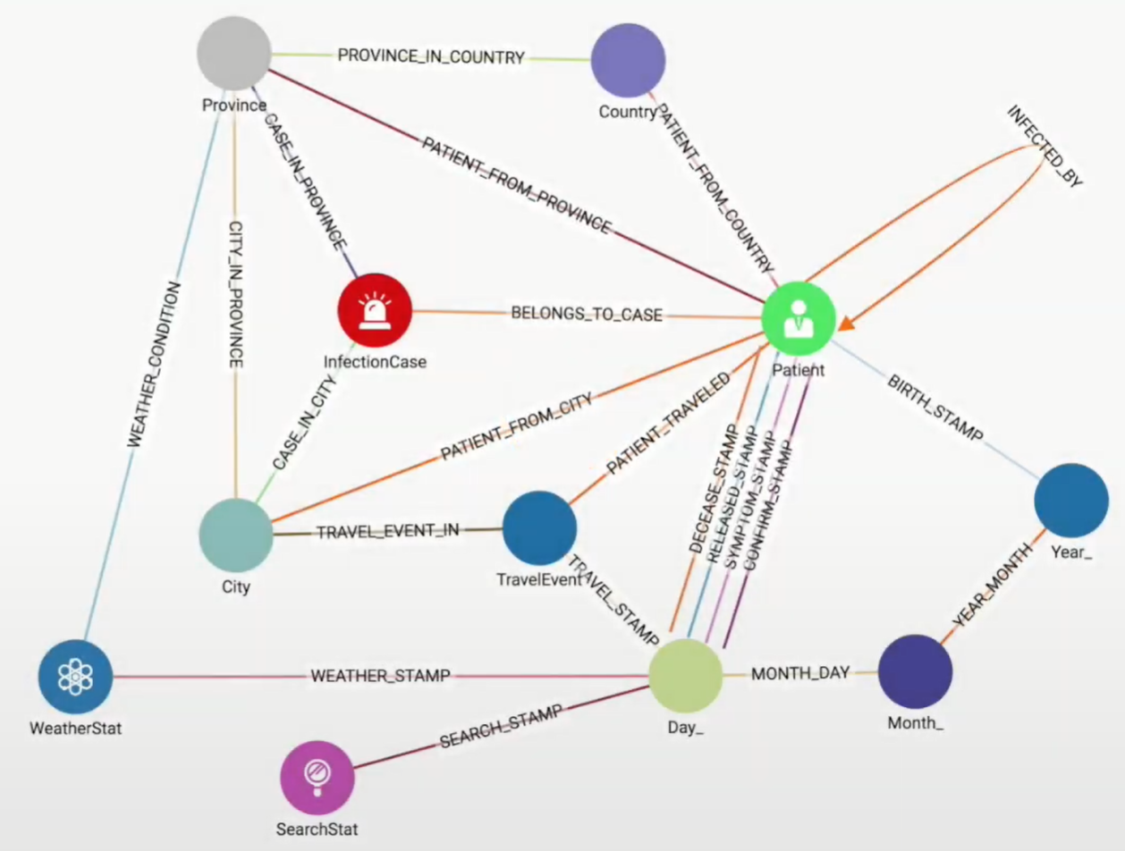
Figure 1-11. Graph schema for South Korean COVID-19 contact tracing data
With this vertex- and edge-type awareness you can refine some of the domain-independent searches. For example, while you can run PageRank on any graph, the scores will only have significance if all the edges have the same or relatively similar meanings. It would not make sense to run PageRank on the entire COVID-19 contact tracing graph. It would make sense, however, to consider only the Patient vertices and INFECTED_BY edges. PageRank would then tell you who was the most influential Patient in terms of causing infection: Patient zero, so to speak.
In this type of scenario, you also want to apply your understanding of the domain to think of small patterns with two or more edges of specific types that indicate something meaningful. For this COVID-19 contact tracing schema, the most important facts are Infection Status (InfectionCase), Who (Patient), Where (City and TravelEvent) and When (Day_). Paths that connect these are important. A possible feature is “number of travel events made by Patient P in March 2020.” A more specific feature is “number of Infected Patients in the same city as Patient P in March 2020.” That second feature is the type of question we posed in the Analyze section of our book. You’ll find examples of vertex and edge type-specific PageRank and domain-dependent pattern queries in the TigerGraph Cloud Starter Kit for COVID-19.
Let’s pause for a minute to reflect on your immediate goal for extracting these features. Do you expect these features to directly point out actionable situations, or are you building a collection of patterns to feed into a machine learning system? The machine learning system will then tell you which features matter, to what degree, and in what combination. If you’re doing the latter, which is our focus for this chapter, then you don’t need to build overly complex features. Instead, focus on building block features. Try to include some that provide a number (e.g., how many travel events) or a choice among several possibilities (e.g., city most visited).
To provide a little more inspiration for using graph-based features, here are some examples of domain-dependent features used in real-world systems to help detect financial fraud:
-
How many shortest paths are there between a loan applicant and a blacklisted entity, up to a maximum path length (because very long paths represent negligible risk)?
-
How many times has the loan applicant’s mailing address, email address, or phone number been used by differently named applicants?
-
How many credit card charges has this card made in the last 10 minutes?
While it is easy to see that high values on any of these measures make it more likely that a situation involves financial misbehavior, our goal is to be more precise and more accurate. We want to know what are the threshold values, and what about combinations of factors? Being precise cuts down on false negatives (missing cases of real fraud) and cuts down on false positives (labeling a situation as fraud when it really isn’t). False positives are doubly damaging. They hurt the business because they are rejecting an honest business transaction, and they hurt the customer who has been unjustly labeled a crook.
Graph Embeddings: A Whole New World
Our last approach to feature extraction is graph embedding, a hot topic of research and discussion of late. Some authorities may find it unusual that I am classifying graph embedding as a type of feature extraction. Isn’t graph embedding a kind of dimensionality reduction? Isn’t it representation learning? Isn’t it a form of machine learning itself? All of those are true. Let’s first define what is a graph embedding.
An embedding is a representation of a topological object in a particular system such that the properties we care about are preserved (or approximated well). The last part “the properties we care about are preserved” speaks to why we use embeddings. A well-chosen embedding makes it more convenient to see what we want to see.
Here are several examples to help illustrate the meaning of embeddings:
-
The earth is a sphere but we print world maps on flat paper. The representation of the earth on paper is an embedding. There are several different standard representations or embeddings of the earth as a map. Figure 1-12 shows some examples.
-
Prior to the late 2010s, when someone said graph embedding, they probably meant something like the earth example. To represent all the connections in a graph without edges touching one another, you often need three or more dimensions. Whenever you see a graph on a flat surface, it’s an embedding, as in Figure 1-13. Moreover, unless your data specifies the location of vertices, then even a 3-D representation is an embedding because it’s a particular choice about the placement of the vertices. From a theoretical perspective, it takes up to n-1 dimensions to represent a graph with n vertices: huge!
-
In natural language processing (NLP), a word embedding is a sequence of scores (i.e., a feature vector) for a given word (see Figure 1-14). There is no natural interpretation of the individual scores, but an ML program sets the scores so that words that tend to occur near each other in training documents have similar embeddings. For example, “machine” and “learning” might have similar embeddings. A word embedding is not convenient for human use, but it is very convenient for computer programs that need a computational way of understanding word similarities and groupings.
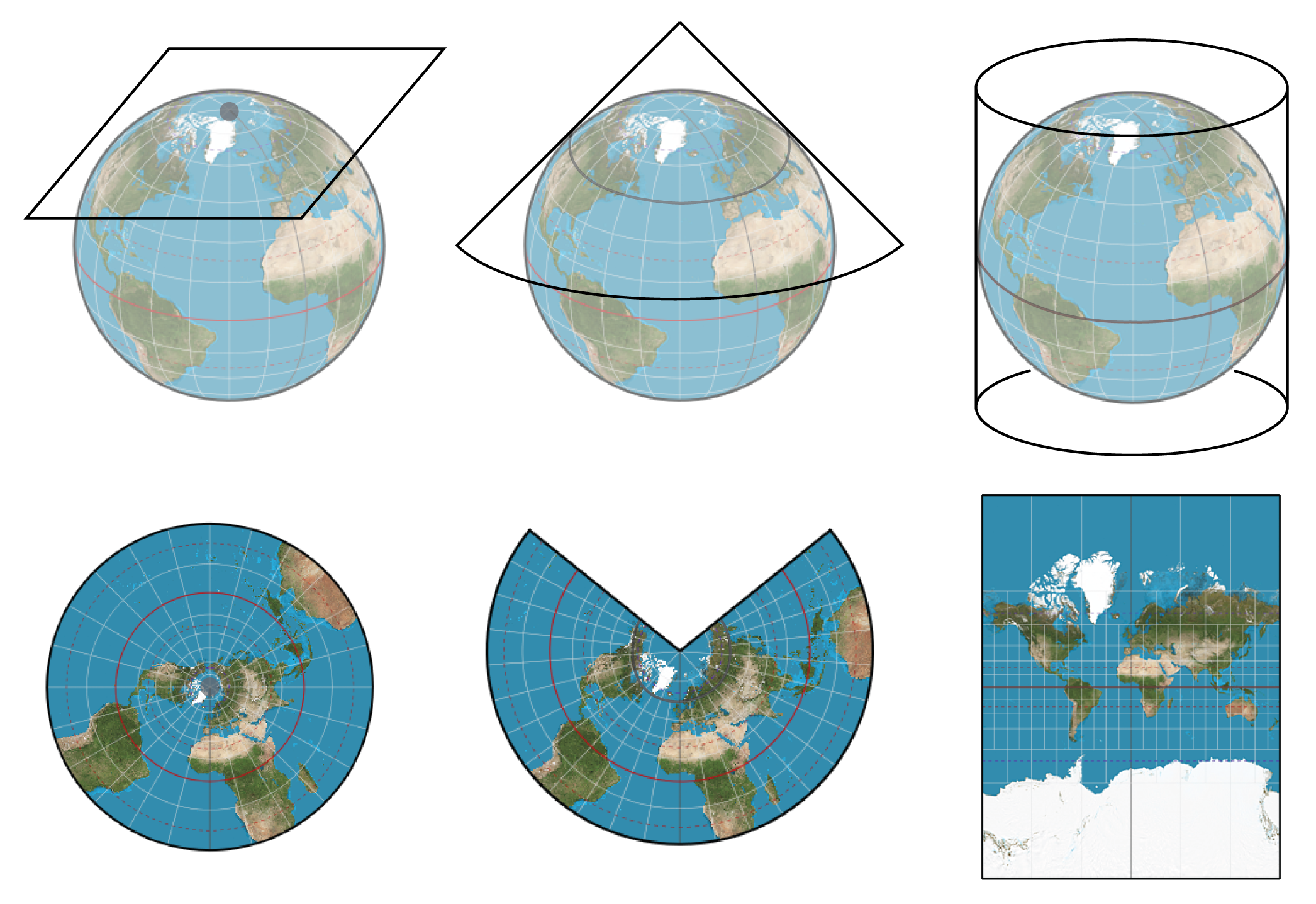
Figure 1-12. Two embeddings of the earth’s surface onto 2-D space9
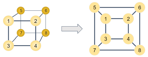
Figure 1-13. Some graphs can be embedded in 2-D space without intersecting edges

Figure 1-14. Word embedding
In recent years, graph embedding has taken on a new meaning, analogous to word embedding. We compute one or more feature vectors to approximate the graph’s neighborhood structure. In fact, when people say graph embedding, they often mean vertex embedding: computing a feature vector for each vertex in the graph. A vertex’s embedding tells us something about how it connects to others. We can then use the collection of vertex embeddings to approximate the graph, no longer needing to consider the edges. There are also methods to summarize the whole graph as one embedding. This is useful for comparing one graph to another. In this book, we will focus on vertex embeddings.
Figure 1-15 shows an example of a graph (a) and portion of its vertex embedding (b). The embedding for each vertex (a series of 64 numbers) describes the structure of its neighborhood without directly mentioning any of its neighbors.

Figure 1-15. (a) Karate club graph10 and (b) 64-element embedding for two of its vertices
Let’s return to the question of classifying graph embeddings. As we will see, the technique of graph embedding requires unsupervised learning, so it can also be considered a form of representation learning. What graph embeddings give us is a set of feature vectors. For a graph with a million vertices, a typical embedding vector would be a few hundred elements long, a lot less than the upper limit of one million dimensions. Therefore, graph embeddings also represent a form of dimensionality reduction. And, we’re using graph embeddings to get feature vectors, so they’re also a form of feature extraction.
Does any feature vector qualify as an embedding? That depends on whether your selected features are telling you what you want to know. Graphlets come closest to the learned embeddings we are going to examine because of the methodical way they deconstruct neighborhood relationships.
Random Walk-based Embeddings
One of the best known approaches for graph embedding is to use random walks to get a statistical sample of the neighborhood surrounding each vertex v. A random walk is a sequence of connected hops in a graph G. The walk starts at some vertex v. It then picks a random neighbor of v and moves there. It repeats this selection of random neighbors until it is told to stop. In an unbiased walk, there is an equal probability of selecting any of the outgoing edges.
Random walks are great because they are easy to do and gather a lot of information efficiently. All feature extraction methods we have looked at before require following careful rules about how to traverse the graph; graphlets are particularly demanding due to their very precise definitions and distinctions from one another. Random walks are carefree. Just go.
For the example graph in Figure 1-16, suppose we start a random walk at vertex A. There is an equal probability of 1 in 3 that we will next go to vertex B, C, or D. If you start the walk at vertex E, there is a 100% chance that the next step will be to vertex B. There are variations of the random walk rules where there’s a chance of staying in place, reversing your last step, jumping back to the start, or jumping to a random vertex.

Figure 1-16. An ordinary graph for leisurely walks
Each walk can be recorded as a list of vertices, in the order in which they were visited. A-D-H-G-C is a possible walk. You can think of each walk as a signature. What does the signature tell us? Suppose that walk W1 starts at vertex 5 and then goes to 2. Walk W2 starts at vertex 9 and then goes to 2. Now they are both at 2. From here on, they have exactly the same probabilities for the remainder of their walks. Those individual walks are unlikely to be the same, but if there is a concept of a “typical walk” averaged over a sampling of several walks, then yes, the signatures of 5 and 9 would be similar. All because 5 and 9 share a neighbor 2. Moreover, the “typical walk” of vertex 2 itself would be similar, except offset by one step.
It turns out that these random walks gather neighborhood information much in the same way that SimRank and RoleSim gather theirs. The difference is that those role similarity algorithms considered all paths (by considering all neighbors), which is computationally expensive. SimRank and RoleSim differ from one another in how they aggregate the neighborhood information. Let’s take a look at two random-walk based graph embedding algorithms that use a completely different computational method, one borrowed from neural networks.
DeepWalk
The DeepWalk algorithm (Perozzi et al. 2014) collects k random walks of length λ for every vertex in the graph. If you happen to know the word2vec algorithm (Mikolov et al. 2013), the rest is easy. Treat each vertex like a word and each walk like a sentence. Pick a window width w for the skip-grams and a length d for your embedding. You will end up with an embedding (latent feature vector) of length d for each vertex. The DeepWalk authors found that k=30 walks, walk length λ=40, with window width w=10 and embedding length d=64 worked well for their test graphs. Your results may vary. Figure 1-17(a) shows an example of a random walk, starting at vertex C and with a length of 16, which is 15 steps or hops from the starting point. The shadings will be explained when we explain skip-grams.

Figure 1-17. (a) Random walk vector and (b) a corresponding skip-gram
We assume you don’t know word2vec, so we’ll give a high-level explanation, enough so you can appreciate what is happening. This is the conceptual model. The actual algorithm plays a lot of statistical tricks to speed up the work. First, we construct a simple neural network with one hidden layer, as shown in Figure 1-18. The input layer accepts vectors of length n, where n = number of vertices. The hidden layer has length d, the embedding length because it is going to be learning the embedding vectors. The output layer also has length n.
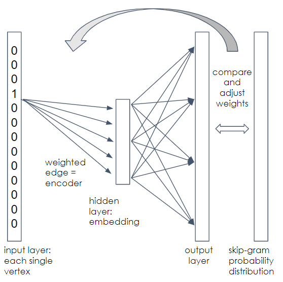
Figure 1-18. Neural network for DeepWalk
Each vertex needs to be assigned a position in the input and output layer, e.g., vertex A is at position 1, vertex B is at position 2, etc. Between the layers are two meshes of n ✕ d connections, from each element in one layer to each element in the next layer. Each edge has a random weight initially, but we will gradually adjust the weights of the first mesh.
Start with one walk for one starting vertex. At the input, we represent the vertex using one-hot encoding. The vector element that corresponds to the vertex is set to 1; all other elements are set to 0. We are going to train this neural network to predict the neighborhood of the vertex given at the input.
Applying the weights in the first mesh to our one-hot input, we get a weighted vertex in the hidden layer. This is the current guess for the embedding of the input vertex. Take the values in the hidden layers and multiply by the weights of the second mesh to get the output layer values. You now have a length-n vector with random weights.
We’re going to compare this output vector with a skip-gram representation of the walk. This is where we use the window parameter w. For each vertex in the graph, count how many times it appears within w-steps before or after the input vertex v. We’ll skip the normalization process, but your final skip-gram vector expresses the relative likelihood that each of the n vertices is near vertex v in this walk. Now we’ll explain the result of Figure 1-17. Vertex C was the starting point for the random walk; we’ve used dark shading to highlight every time we stepped on vertex C. The light shading shows every step that is within w = 2 steps of vertex C. Then, we form the skip-gram in (b) by counting how many times we set foot on each vertex within the shaded zones. For example, vertex G was stepped on twice, so the skip-gram has 2 in the position for G. This is a long walk on a small graph, so most vertices were stepped on within the windows. For short walks on big graphs, most of the values will be 0.
Our output vector was supposed to be a prediction of this skip-gram. Comparing each position in the two vectors, if the output vector’s value is higher than the skip-gram’s value, then lower the corresponding weight in the input mesh. If the value was lower, then raise the corresponding weight.
You’ve processed one walk. Repeat this for one walk of each vertex. Now repeat for a second walk of each vertex, until you’ve adjusted your weights for k ✕ n walks. You’re done! The weights of the first n ✕ d mesh are the length-d embeddings for your n vectors. What, about the second mesh? Strangely, we were never going to directly use the output vectors, so we didn’t bother to adjust its weight.
Here is how to interpret and use a vertex embedding:
-
For neural networks in general, you can’t point to a clear real-world meaning of the individual elements in the latent feature vector.
-
Based on how we trained the network, though, we can reason backwards from the skip-grams, which represent the neighbors around a vertex: vertices that have similar neighborhoods should have similar embeddings.
-
If you remember the example earlier about two paths that were offset by one step, note that those two paths would have very similar skip-grams. So, vertices that are close to each other should have similar embeddings.
One critique of DeepWalk is that its uniformly random walk is too random. In particular, it may wander far from the source vertex before getting an adequate sample of the neighborhoods closer to the source. One way to address that is to include a probability of resetting the walk by magically teleporting back to the source vertex and then continuing with random steps again, as in Zhou et al. 2021. This is known as “random walk with restart”.
Node2vec
Another method which has already gained popularity is node2vec [Grover and Leskovec 2016]. It uses the same skip-gram training process as DeepWalk, but it gives the user two adjustment parameters to control the direction of the walk: go farther (depth), go sideways (breadth), or go back a step. Farther and back seem obvious, but what exactly does sideways mean?
Suppose we start at vertex A of the graph in Figure 1-19. Its neighbors are vertices B, C, and D. Since we are just starting, any of the choices would be moving forward. Let’s go to vertex C. For the second step, we can choose from any of vertex C’s neighbors: A, B, F, G, or H.

Figure 1-19. Illustrating the biased random walk with memory used in node2vec
If we remember what our choices were in our previous step, we can classify our current set of neighbors into three groups: back, sideways, and forward. We also assign a weight to each connecting edge, which represents the unnormalized probability of selecting that edge.
- Back
-
In our example: vertex A. Edge weight = 1/p.
- Sideways
-
These are the vertices that were available last step and are available this step (e.g., the union of the two sets of vertices. So, they represent a second chance to visit a different neighbor of where you were previously. In our example: vertex B. Edge weight = 1.
- Forward
-
There are all the vertices that don’t return or go sideways. In our example: vertices F, G, and H. Edge weight = 1/q.
If we set p = q = 1, then all choices have equal probability, so we’re back to an unbiased random walk. If p < 1, then returning is more likely than going sideways. If q < 1, then each of the forward (depth) options is more likely than sideways (breadth). Returning also keeps the walk closer to home (e.g., similar to breadth-first-search), because if you step back and then step forward randomly, you are trying out the different options in your previous neighborhood.
This ability to tune the walk makes node2vec more flexible than DeepWalk, which results in better models in many cases.
Besides the random walk approach, there are several other techniques for graph embedding, each with their advantages and disadvantages: matrix factorization, edge reconstruction, graph kernel, and generative models. Though already a little dated, A Comprehensive Survey of Graph Embedding: Problems, Techniques, and Applications, by Cai et al. provides a thorough overview with several accessible tables which compare the features of different techniques.
Summary
Graphs can provide additional and valuable features to describe and understand your data. Key takeaways from this section are as follows:
-
A graph feature is a characteristic that is based on the pattern of connections in the graph
-
Graphlets and centrality algorithms provide domain-independent features for any graph.
-
Applying some domain knowledge to guide your feature extraction leads to more meaningful features.
-
Machine learning can produce vertex embeddings which encode vertex similarity and proximity in terms of compact feature vectors.
-
Random walks are a simple way to sample a vertex’s neighborhood.
Graph Neural Networks
In the popular press, it’s not AI unless it uses a neural network, and it’s not machine learning unless it uses deep learning. Neural networks were originally designed to emulate how the human brain works, but they evolved to address the capabilities of computers and mathematics. The predominant models assume that your input data is in a matrix or tensor; it’s not clear how to present and train the neural network with interconnected vertices. Yet, are there graph-based neural networks? Yes!
Graph neural networks (GNNs) are conventional neural networks with an added twist for graphs. Just as there are several variations of neural networks, there are several variations of GNNs. The simplest way to include the graph itself into the neural network is through convolution.
Graph Convolutional Networks
In mathematics, convolution is how two functions affect the result if one acts on the other in a particular way. It is often used to model situations in which one function describes a primary behavior and another function describes a secondary effect. For example, in image processing, convolution takes into account neighboring pixels to improve identification of boundaries and to add artificial blur. In audio processing, convolution is used to both analyze and synthesize room reverberation effects. A convolutional neural network (CNN) is a neural network that includes convolution in the training process. For example, you could use a CNN for facial recognition. The CNN would systematically take into account neighboring pixels, an essential duty when analyzing digital images.
A graph convolutional network (GCN) is a neural network that uses graph traversal as a convolution function during the learning process. While there were some earlier related works, the first model to distill the essence of graph convolution into a simple but powerful neural network was presented in 2017 with "Semi-Supervised Classification with Graph Convolutional Networks" by Thomas Kipf and Max Welling.
For graphs, we want the embedding for each vertex to include information about the relationships to other vertices. We can use the principle of convolution to accomplish this. Figure 1-20 shows a simple convolution function, with a general model at top and a more specific example at bottom.
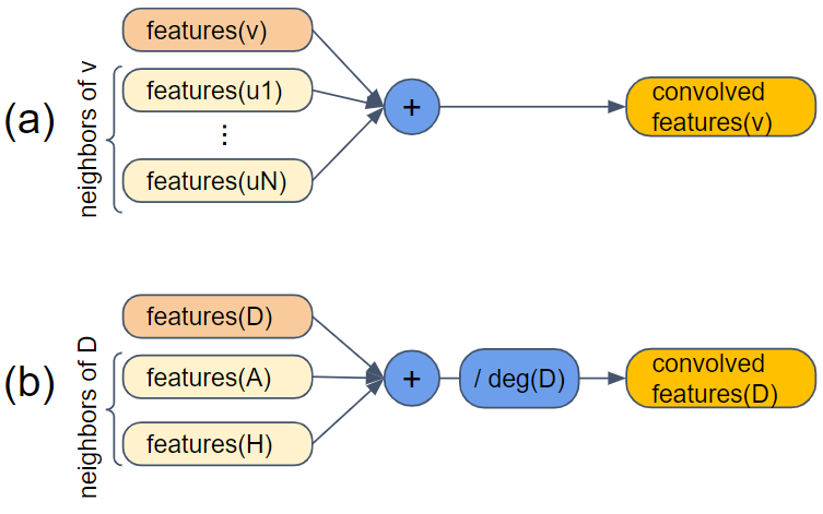
Figure 1-20. Convolution using neighbors of a vertex
In part (a) of the figure, the primary function is features(v): given a vertex v, output its feature vector. The convolution is to combine the features of v with the features of all of the neighbors of v: u1, u2,...,uN. If the features are numeric, we can just add them. The result is the newly convolved features of v. In part (b), we set v = D. Vertex D has two neighbors, A and H. We insert one more step after summing the feature vectors: divide by the degree of the primary vertex. Vertex D has 2 neighbors, so we divide by 2. This regularizes the output values so that they don’t keep getting bigger and bigger. (Yes, technically we should divide by deg(v)+1, but the simpler version seems to be good enough.)
Let’s do a quick example:
features[0](D) = [3, 1 ,4, 1]
features[0](A) = [5, 9, 2, 6]
features[0](H) = [5, 3, 5, 8]
features[1](D) = [6.5, 6.5, 5.5, 7.5]
By having neighbors share their feature values, this simple convolution function performs selective information sharing: it determines what is shared (features) and by whom (neighbors). A neural network which uses this convolution function will tend to evolve according to these maxims:
-
Vertices which share many neighbors will tend to be similar.
-
Vertices which share the same initial feature values will tend to be similar.
These properties are reminiscent of random-walk graph embeddings, aren’t they? But we won’t be using any random walks.
How do we take this convolution and integrate it into a neural network? Take a look at Figure 1-21.
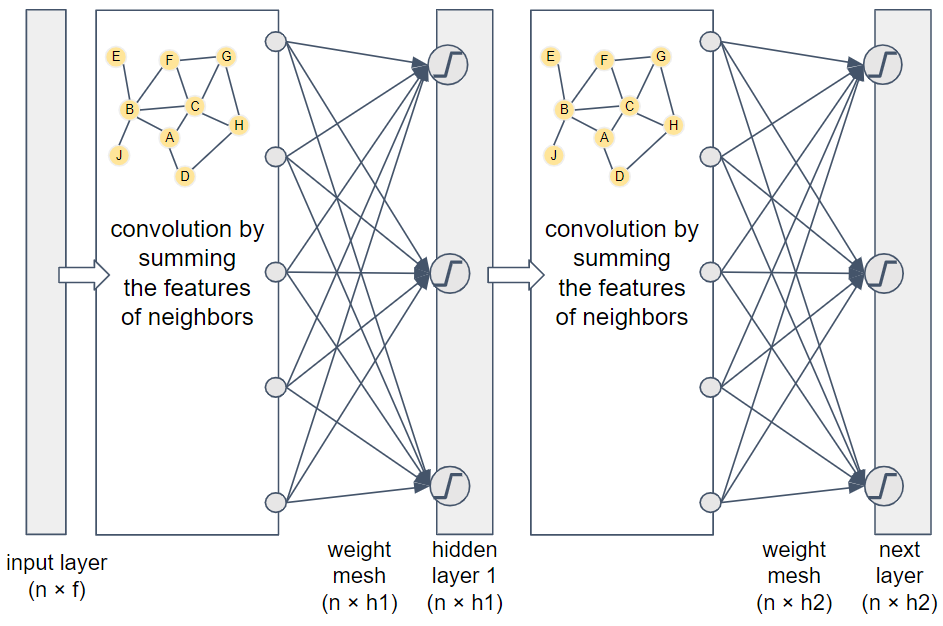
Figure 1-21. Two-layer graph convolutional network
This two-layer network flows from left to right. The input is the feature vectors for all of the graph’s vertices. If the feature vectors run horizontally and we stack the vertices vertically, then we get an n ✕ f matrix, where f is the number of features. Next we apply the adjacency-based convolution. We then apply a set of randomized weights (similar to what we did with random-walk graph embedding networks) to merge and reduce the features to an embedding of size h1. Typically h1 < f. Before storing the values in the embedding matrix, we apply an activation function (indicated by the blocky “S” in a circle) which acts as a filter/amplifier. Low values are pushed lower, and high values are pushed higher. Activation functions are used in most neural networks.
Because this is a two-layer network, we repeat the same steps. The only differences are that this embedding may have a different size, where typically h2 ≤ h1, and this weight mesh has a different set of random weights. If this is the final layer, then it’s considered the output layer with the output results. By having two layers, the output embedding for each vertex takes into account the neighbors within two hops. You can add more layers to consider deeper neighbors. Two or three layers often provide the best results. With too many layers, the radius of each vertex’s neighborhood becomes so large that it overlaps significantly even with the neighborhoods of unrelated vertices.
Our example here is demonstrating how a GCN can be used in unsupervised learning mode. No training data or target function was provided; we just merged features of vertices with their neighbors. Surprisingly, you can get useful results from an unsupervised, untrained GCN. The authors of GCN experimented with a 3-layer untrained GCN, using the well-known Karate Club dataset.They set the output layer’s embedding length of 2, so that they could interpret the two values as coordinate points. When plotted, the output data points showed community clustering which matched the known communities in Zachary’s Karate Club.
The GCN architecture is general enough to be used for unsupervised, supervised, semi-supervised, or even reinforcement learning. The only difference between a GCN and a vanilla feed-forward NN is the addition of the step to aggregate the features of a vector with those of its neighbors. Figure 1-22 shows a generic model for how neural networks tune their weights. The graph convolution in GCN affects only the block labeled Forward Propagation Layers. All of the other parts (input values, target values, weight adjustment, etc.) are what determine what type of learning you are doing. That is, the type of learning is decided independently from your use of graph convolution.
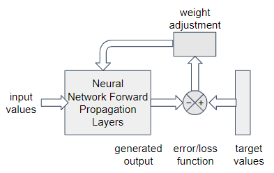
Figure 1-22. Generic model for responsive learning in a neural network
Attention neural networks use a more advanced form of feedback and adjustment. The details are beyond the scope of this book, but graph attention neural networks (GATs) can tune the weight (aka focus the attention) of each neighbor when adding them together for convolution. That is, a GAT performs a weighted sum instead of a simple sum of neighbor’s features, and the GAT trains itself to learn the best weights. When applied to the same benchmark tests, GAT outperforms GCN slightly.
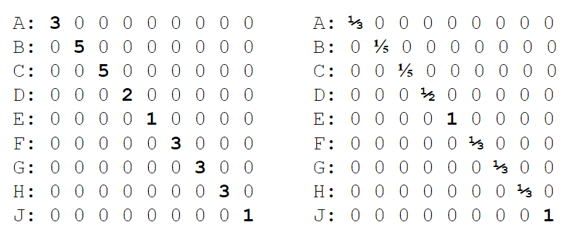
Figure 1-24. The degree matrix D and itself inverse matrix D-1
GraphSAGE
One limitation of the basic GCN model is that it does a simple averaging of vertex + neighbor features. It seems we would want some more control and tuning of this convolution. Also, large variations in the number of neighbors for different vertices may lead to training difficulties. To address this limitation, Hamilton et al. presented GraphSAGE in 2017 in their paper "Inductive Representation Learning on Large Graphs“. Like GCN, this technique also combines information from neighbors, but it does it a little differently. In order to standardize the learning from neighbors, GraphSAGE samples a fixed number of neighbors from each vertex. Figure 1-25 shows a block diagram of GraphSAGE, with sampled neighbors.

Figure 1-25. Block diagram of GraphSAGE
With GraphSAGE, the features of the neighbors are combined according to a chosen aggregation function. The function could be addition, as in GCNs. Any order-independent aggregation function could be used; LSTM with random ordering and max-pooling work well. The source vertex is not included in the aggregation as it is in GCN; instead, the aggregated feature vectors and the source vertex’s feature vector are concatenated to make a double-length vector. We then apply a set of weights to mix the features together, apply an activation function, and store as the next layer’s representation of the vertices. This series of sets constitutes one layer in the neural network and the gathering of information within one hop of each vertex. A GraphSAGE network has k layers, each with its own set of weights. GraphSAGE proposes a loss function that rewards nearby vertices if they have similar embeddings, while rewarding distant vertices if they have dissimilar embeddings.
Besides training on the full graph, as you would with GCN, you can train GraphSAGE with only a sample of the vertices. The fact that GraphSAGE’s aggregation functions uses equally-sized samples of neighborhoods means that it doesn’t matter how you arrange the inputs.That freedom of arrangement is what allows you to train with one sample and then test or deploy with a different sample. Because it can learn from a sample, GraphSAGE performs inductive learning. In contrast, GCN directly uses the adjacency matrix, which forces it to use the full graph with the vertices arranged in a particular order. Training with the full data and learning a model for only that data is transductive learning.
Whether learning from a sample will work on your particular graph depends on whether your graph’s structure and features follow global trends, such that a random subgraph looks similar to another subgraph of similar size. For example, one part of a forest may look a lot like another part of a forest. For a graph example, suppose you have a Customer 360 graph including all of a customer’s interactions with your sales team, website, events, their purchases, and all other profile information you have been able to obtain. Last year’s customers are rated based on the total amount and frequency of their purchases. It is reasonable to expect that if you used GraphSAGE with last year’s graph to predict the customer rating, it should do a decent job of predicting the ratings of this year’s customers. Table 1-4 summarizes all the similarities and differences between GCN and GraphSAGE that we have presented.
| GCN | GraphSAGE | |
| Neighbors for aggregation | All | sample of n neighbors |
| Aggregation function | mean | several options |
| Aggregating a vertex with neighbors? | aggregated with others | concatenated to others |
| Do weights need to be learned? | not for unsupervised transductive model | yes, for inductive model |
| Unsupervised? | yes | yes |
| Supervised? | with modification | with modification |
| Can be trained on a sample of vertices | no | yes |
Summary
Graph-based neural networks put graphs into the mainstream of machine learning. Key takeaways from this section are as follows:
-
The graph convolutional neural network (GCN) enhances the vanilla neural network by averaging together the feature vectors of each vertex’s neighbors with its own features during the learning process.
-
GraphSAGE makes two key improvements to the basic GCN: vertex and neighborhood sampling, and keeping features of vectors separate from those of its neighbors .
-
GCN learns transductively (uses the full data to learn only about that data) whereas GraphSAGE learns inductively (uses a data sample to learn a model that can apply to other data samples).
-
The modular nature of neural networks and graph enhancements mean that the ideas of GCN and GraphSAGE can be transferred to many other flavors of neural networks.
Comparing Graph Machine Learning Approaches
This chapter has covered many different ways to learn from graph data, but it only scratched the surface. Our goal was not to present an exhaustive survey, but to provide a framework from which to continue to grow. We’ve outlined the major categories of and techniques for graph-powered machine learning, we’ve described what characterizes and distinguishes them, and we’ve provided simple examples to illustrate how they operate. It’s worthwhile to briefly review these techniques. Our goal here is not only to summarize but also to provide you with guidance for selecting the right techniques to help you learn from your connected data.
Use Cases for Machine Learning Tasks
Table 1-5 pulls together examples of use cases for each of the major learning tasks. These are the same basic data mining and machine learning tasks you might perform on any data, but the examples are particularly relevant for graph data.
| Task | Use case examples |
| Community detection | Delineating social networks |
| Finding a financial crime network | |
| Detecting an biological ecosystem or chemical reaction network | |
| Discovering a network of unexpectedly interdependent components or process, such as software procedures or legal regulations | |
| Similarity | Abstraction of physical closeness, inverse of distance |
| Prerequisite for clustering, classification, and link prediction | |
| Entity resolution - finding two online identities that probably refer to the same real-world person | |
| Product recommendation or suggested action | |
| Identifying persons who perform the same role in different but analogous networks | |
| Find unknown patterns | Identifying the most common “customer journeys” on your website or in your app |
| Discovering that two actions - planning a summer vacation and | |
| Once current patterns are identified, then noticing changes | |
| Link Prediction | Predicting someone’s future purchase or willingness to purchase |
| Predicting that business or personal relationship exists, even though it is not recorded in the data | |
| Feature Extraction | Enriching your customer data with graph features, so that your ML training to categorize and model your customers will be more successful |
| Embedding | Transforming a large set of features to a more compact set, for more efficient computation |
| Classification (predicting a category) | Given some past examples of fraud, create a model for identifying new cases of fraud |
| Predicting categorical outcomes for future vaccine patients, based on test results of past patients | |
| Regression (predicting a numerical value) | Predicting weight loss for diet program participants, based on results of past participants |
Once you have identified what type of task you want to perform, consider the available graph-based learning techniques, what they provide, and their key strengths and differences.
Graph-based Learning Methods for Machine Learning Tasks
Table 1-6 lists the graph algorithms and feature extraction methods which we encountered in the chapter. Table 1-7 compares graph neural network methods.
| Task | Graph-based Learning Methods | Comments |
| Community detection | connected components | one connection to the community is enough |
| k-core | at least k connections to other community members | |
| modularity optimization, e.g. Louvain | relatively higher density of connections inside than between communities | |
| Similarity | Jaccard neighborhood similarity | counts how many relationships in common, for nonnumeric data |
| cosine neighborhood similarity | compares numeric or weighted vectors of relationships | |
| role similarity | defines similarity recursively as having similar neighbors | |
| Find unknown patterns | frequent pattern mining | starts with small patterns and builds to larger patterns |
| Domain- independent feature extraction | graphlets | systematic list of all possible neighborhood configurations |
| PageRank | rank is based on the number and rank of in-neighbors, for directed graphs among vertices of the same type | |
| closeness centrality | closeness = average distance to any other vertex | |
| betweenness centrality | how often a vertex lies on the shortest path between any two vertices; slow to compute | |
| Domain- dependent feature extraction | searching for patterns relevant to your domain | custom effort by someone with domain knowledge |
| Dimensionality reduction and embedding | DeepWalk | embeddings will be similar if the vectors have similar random walks, considering nearness and role; more efficient than SimRank |
| node2vec |
DeepWalk with directional tuning of the random walks, for greater tuning |
Graph Neural Networks: Summary and Uses
The graph neural networks presented in this chapter not only are directly useful in many cases but also templates to show more advanced data scientists how to transform any neural network technique to include graph connectivity in the training. The key is the convolution step, which takes the features of neighboring vertices into account. All of the graph neural network approaches presented can be used for either unsupervised or supervised learning.
| Name | Description | Uses |
| Graph Convolutional Network (GCN) | Convolution: average of neighbor’s features | Clustering or classification on a particular graph |
| GraphSAGE | Convolution: average of a sample of neighbor’s features | learning a representative model on a sample of a graph, in addition to clustering or classification |
| Graph Attention Network (GAT) | Convolution: weighted average of neighbor’s features | clustering, classification, and model learning; added tuning and complexity by learning weights for the convolution |
Chapter Summary
Graphs and graph-based algorithms contribute to several stages of the machine learning pipeline: data acquisition, data preparation, feature extraction, dimensionality reduction, and model training. As data scientists know, there is no golden ticket, no single technique that solves all their problems. Instead, you work to acquire tools for your toolkit, develop the skills to use your tools well, and gain an understanding about when to use them.
1 The use of a table for our small example may suggest that a graph structure is not needed. We assume you already decided to organize your data as a graph and now are analyzing and learning from that data.
2 One of the authors of this book, Victor Lee, is a coauthor of RoleSim.
3 A hop is the generic unit of distance in a graph, from one vertex to its neighbor. We defined this in Chapter 1.
4 Graphlets were first presented by Nataša Pržulj et al. in "Modeling interactome: scale-free or geometric?“.
5 "Graphlet-based Characterization of Directed Networks“, Sarajlić et al., 2016.
6 "Link Prediction in Dynamic Networks using Graphlet”, Rahmat et al., 2016.
7 From "Uncovering Biological Network Function via Graphlet Degree Signatures" by Tijana Milenković
and Nataša Pržulj, licensed under CC BY 3.0
8 These algorithms were introduced in the Analyze section of the book.
9 From Battersby, S. (2017). Map Projections. The Geographic Information Science & Technology Body of Knowledge (2nd Quarter 2017 Edition), John P. Wilson (ed.). DOI: 10.22224/gistbok/2017.2.7
10 Visualized partitioning of Zachary’s Karate Club, licensed under CC BY_SA 4.0