Chapter 7. Designing Applications with Cassandra
In the previous chapters you learned how Cassandra represents data, how to create Cassandra data models, and how Cassandra’s architecture works to distribute data across a cluster so that we can access it quickly and reliably. Now it’s time to take this knowledge and start to apply it in the context of real-world application design.
Hotel Application Design
Let’s return to the hotel domain we began working with in Chapter 5. Imagine that we’ve been asked to develop an application that leverages the Cassandra data models we created to represent hotels, their room availability, and reservations.
How will we get from a data model to the application? After all, data models don’t exist in a vacuum. There must be software applications responsible for writing and reading data from the tables that we design. While we could take many architectural approaches to developing such an application, we’ll focus in this chapter on the microservice architectural style.
Cassandra and Microservice Architecture
Over the past several years, the microservice architectural style has been foundational to the discipline of cloud-native applications. As a database designed from the cloud from the ground up, Cassandra is a natural fit for cloud-native applications.
We don’t intend to provide a full discussion of the benefits of a microservice architecture here, but will reference Sam Newman’s book Building Microservices as an excellent source on this topic.
- Encapsulation
-
Encapsulation could also be phrased as “services that are focused on doing one thing well” or the “single responsibility principle”.
By contrast, in many enterprises the database serves as a central integration point. An application might expose interfaces to other applications such as remote procedure call (RPC) or messaging interfaces, but its also common for one application to access another application’s database directly, which violates encapsulation and produces dependencies between applications that can be difficult to isolate and debug.
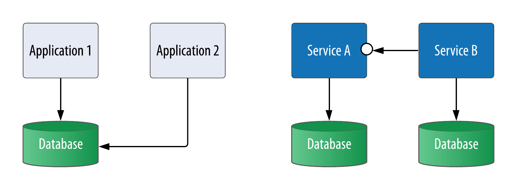
Figure 7-1. Integration by Database contrasted with Microservices
- Autonomy
-
In a microservice architecture, autonomy refers to the ability to independently deploy each microservice without dependence on any other microservices. This flexibility has significant advantages in allowing you to independently evolve portions of a deployed application without downtime, using approaches such as blue/green deployments that allow you to gradually introduce new versions of a service and miminize the risk of these deployments.
Another implication of autonomy is that each microservice can have its own data store using the most appropriate technology for that service. We’ll examine this flexibility in more detail in “Polyglot Persistence” below.
- Scalability
-
Microservice architecture provides a lot of flexibility by giving us the ability to run more or fewer instances of a service dynamically according to demand. This allows us to scale different aspects of an application independently.
For example, in a hotel domain there is a large disparity between shopping (the amount of traffic devoted to looking for hotel rooms) and booking (the much lower level of traffic associated with customers actually committing to a reservation). For this reason, we might expect to scale the services associated with hotel and inventory data to a higher degree than the services associated with storing reservations.
Microservice Architecture for a Hotel Application
To create a microservice architecture for our hotel application, we’ll need to identify services, their interfaces, and how they interact. Although it was written well before microservices became popular, Eric Evans’ book Domain Driven Design has proven to be a useful reference. One of the key principles Evans articulates is beginning with a domain model and identifying bounded contexts. This process has become a widely recommended approach for identifying microservices.
In Figure 7-2, we see some of the key architecture and design artifacts that are often produced when building new applications. Rather than a strict workflow, these are presented in an approximate order. The influences between these artifacts are sometimes sequential or waterfall style, but are more often iterative in nature as designs are refined.

Figure 7-2. Artifacts produced by architectural and design processes
Use cases and access patterns are user experience (UX) design artifacts that also influence the data modeling and software architecture processes. We discussed the special role of access patterns in Cassandra data modeling in Chapter 5, so we’ll focus here on the interactions between data modeling and software architecture.
To define a microservice architecture, we’ll use a process that complements our data modeling processes. As we begin to identify entities as part of a conceptual data modeling phase, we can begin to identify bounded contexts that represent groupings of related entities. As we progress into logical data modeling, we refine the bounded contexts in order to identify specific services that will be responsible for each table (or group of related denormalized tables). During the final stage of the design process we confirm the design of each service, the selection of database, the physical data models, and actual database schema.
Identifying Bounded Contexts
Now that we’ve outlined a high level process, let’s see how it works in practice for our hotel application. Reusing the conceptual data model from Chapter 5, we might choose to identify a Hotel Domain encompassing the information about hotels, their rooms and availability, and a Reservation Domain to include information about reservations and guests, as shown in Figure 7-3. These happen to correspond to the keyspaces we identified in our initial data model.
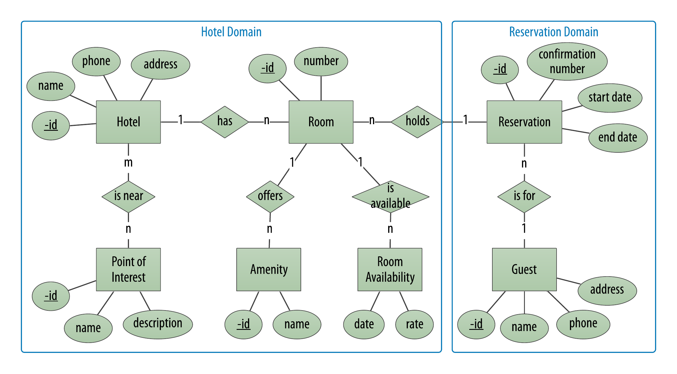
Figure 7-3. Identifying bounded contexts for a hotel application
Identifying Services
The next step is to formalize the bounded contexts we’ve identified into specific services that will own specific tables within our logical data model. For example, the Hotel Domain identified previously might decompose into separate services focused on hotels, points of interest, and inventory availability, as shown in Figure 7-4.

Figure 7-4. Identifying services for hotel data
There are multiple possible designs, but a good general design principle is to assign tables that have a high degree of correspondence to the same service. In particular, when working with Cassandra, a natural approach is to assign denormalized tables representing the same basic data type to the same service.
Services should embody classic object oriented principles of coupling and cohesion: there should be a high degree of cohesion or relatedness between tables owned by a service, and a low amount of coupling or dependence between contexts. The query arrows we drew previously on our Chebotko diagrams are helpful here in identifying relationships between services, whether they are direct invocation dependencies, or data flows orchestrated through user interfaces or events.
Using the same principles as above as we examine the tables in our logical data model within the Reservation Domain, we might identify a Reservation Service and a Guest Service, as shown in Figure 7-5. In many cases there will be a one-to-one relationship between bounded contexts and services, although with more complex domains there could be further decomposition into services.
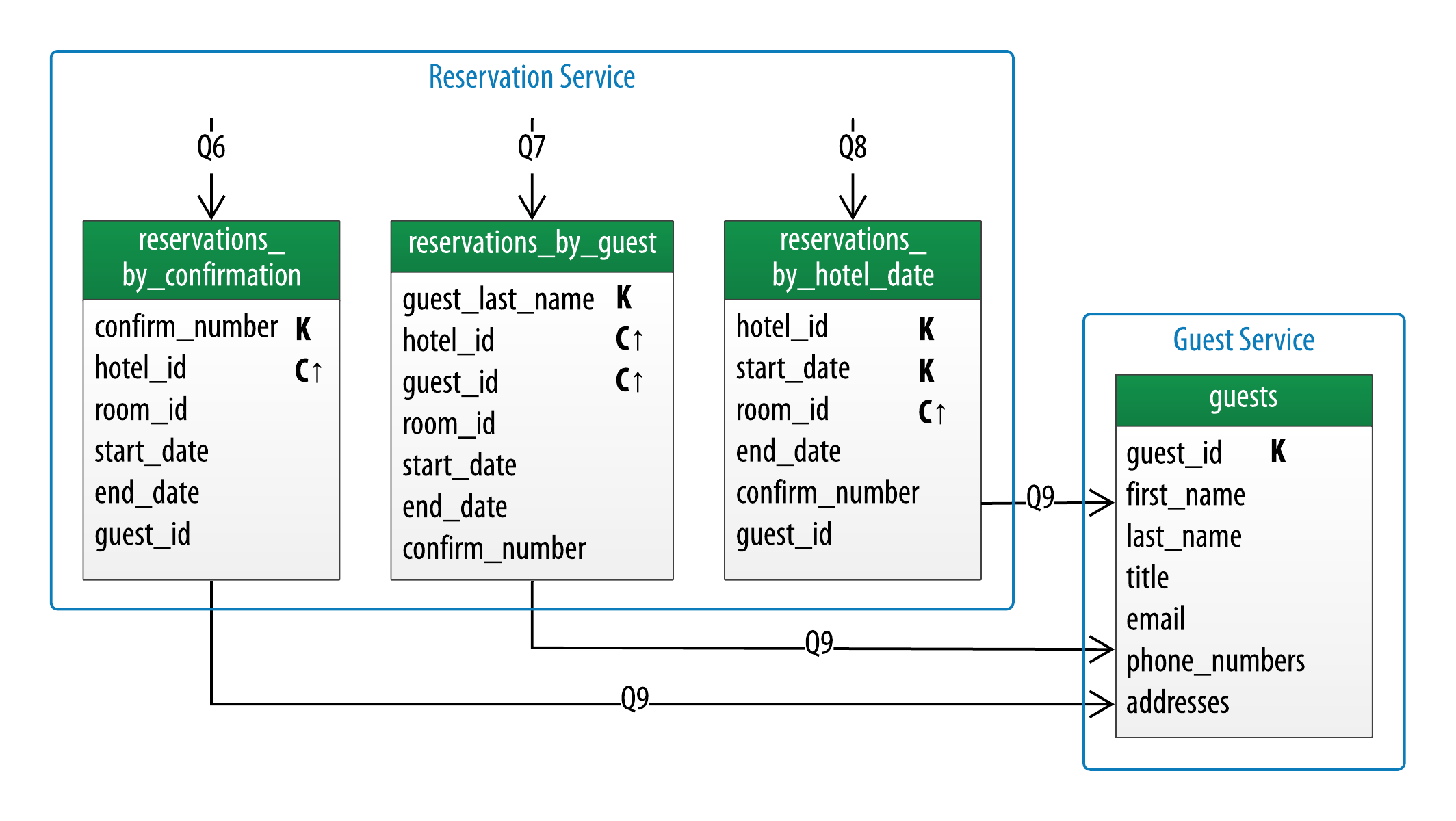
Figure 7-5. Identifying services for reservation data
While our initial design did not specifically identify access patterns for guest data outside of navigating to guest information from a reservation, it’s not a big stretch to imagine that our business stakeholders will at some point want to allow guests to create and manage accounts on our application.
Designing Microservice Persistence
The final stage in our data modeling process consists of creating physical data models. This corresponds to the architectural tasks of designing services; we’ll focus on database-related design choices, including selecting a database and creating database schema.
Polyglot Persistence
One of the benefits of microservice architecture is that each service is independently deployable. This gives us the ability to select a different database for each microservice, an approach known as polyglot persistence.
While you might be surprised to read this in a book on Cassandra, it is nonetheless true that Cassandra may not be the ideal backing store for every microservice, especially those that do not require the scalability that Cassandra offers.
Let’s examine the services we’ve identified in the design of our hotel application to identify some options for polyglot persistence. We’ll summarize these in Table 7-1.
| Service | Data Characteristics | Database Options |
|---|---|---|
Hotel Service |
Descriptive text about hotels and their amenities, changes infrequently |
Document Database (i.e. MongoDB), Cassandra |
Point of Interest Service |
Geographic locations and descriptions of points of interest |
Cassandra or other tabular databases supporting geospatial indexes |
Inventory Service |
Counts of available rooms by date, large volume of reads and writes |
Cassandra or other tabular databases |
Reservation Service |
Rooms reserved on behalf of guests, lower volume of reads and writes than inventory |
Cassandra or other tabular databases |
Guest Service |
Guest identity and contact information, possible extension point for customer and fraud analytics systems |
Cassandra, graph databases |
We might make some of our selections with an eye to future extensibility of the system.
Representing Other Database Models in CQL
When choosing to use Cassandra as the primary underlying database across multiple services, it is still possible to achieve some of the characteristics of other data models such as key-value models, document models, and graph models:
- Key-value models
-
Key-value models can be represented in Cassandra by treating the key as the partition key. The remaining data can be stored in a value column as a text or blob type.
- Document models
-
There are two primary approaches in which Cassandra can behave like a document database, one based on having a well-defined schema, and the other approximating a flexible schema approach. Both involve identifying primary key columns according to standard Cassandra data modeling practices discussed in Chapter 5.
The flexible schema approach involves storing non-primary key columns in a blob, as in the following table definition:
CREATE TABLE hotel.hotels_document (
    id text PRIMARY KEY,
    document text);
With this design, the
documentcolumn could contain arbitrary descriptive data in JavaScript Object Notation (JSON) or some other format, which would be left to the application to interpret. This could be somewhat error-prone and is not a very elegant solution.A better approach is to use CQL support for reading and writing data in JSON format, introduced in Cassandra 2.2. For example, we could insert data into the
hotelstable with this query:cqlsh:hotel> INSERT INTO hotels JSON '{ "id": "AZ123", "name": "Super Hotel Suites at WestWorld", "phone": "1-888-999-9999", "address": { "street": "10332 E. Bucking Bronco", "city": "Scottsdale", "state": "AZ", "zip_code": 85255 } }';Similarly, we can request data in JSON format from a CQL query. The response will contain a single text field labeled
jsonthat includes the requested columns - in this case, all of them (note that no formatting is provided for the output):cqlsh:hotel> SELECT JSON * FROM hotels WHERE id = 'AZ123'; [json] ------------------------------------------------ { "id": "AZ123", "name": "Super Hotel Suites at WestWorld", "phone": "1-888-999-9999", "address": { "street": "10332 E. Bucking Bronco", "city": "Scottsdale", "state": "AZ", "zip_code": 85255 }The
INSERT JSONandSELECT JSONcommands are particularly useful for web applications or other JavaScript applications that use JSON representations. While the ability to read and write data in JSON format does make Cassandra appear to behave more like a document database, remember that all of the referenced attributes must be defined in the table schema. - Graph models
-
Graph data models are a powerful way of representing domains where the relationships between entities are as important or more important than the properties of the entities themselves. Common graph representations include property graphs. A property graph consists of vertexes that represent the entities in a domain, while edges represent the relationships between vertices and can be navigated in either direction. Both vertices and edges can have properties, hence the name property graph.
Property graphs between related entities can be represented on top of Cassandra using an approach in which each vertex type and edge type is stored in a dedicated table. To interact with the graph, applications use a graph query language such as Gremlin or Cypher. Graph databases provide a processing engine that interprets these queries and executes them, including data access to an underlying storage layer. DataStax Graph is an example of a graph database that uses Cassandra as the underlying storage layer.
Extending Designs
Anyone who has built and maintained an application of significant size knows that change is inevitable. Business stakeholders come up with new requirements that cause us to extend systems.
For example, let’s say our business stakeholder approaches us after our initial hotel data model to identify additional ways that customers should be able to search for hotels in our application. We might represent these as additional access patterns, such as searching for hotels by name, location, or amenities, as shown in Figure 7-6.
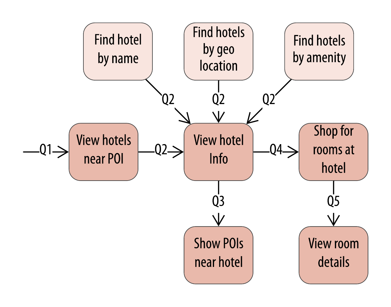
Figure 7-6. Additional hotel access patterns
According to the principles we learned in Chapter 5, our first thought will be to continue our practice of denormalization, creating new tables that will be able to support each of these access patterns, as shown in Figure 7-7.
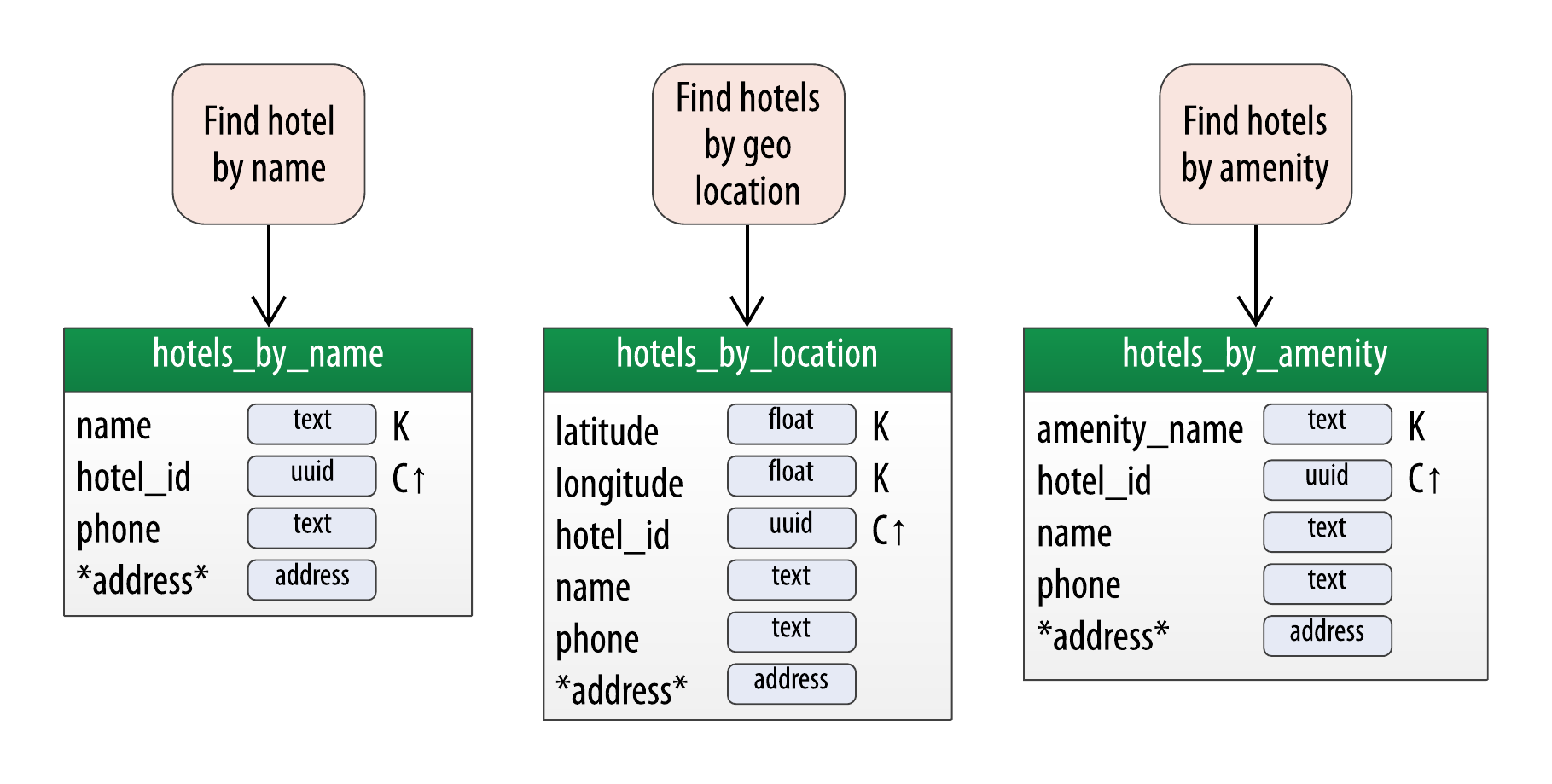
Figure 7-7. Additional hotel tables
At this point, we now have 5 different access patterns for hotel data, and it’s reasonable to begin to ask how many denormalized tables is too many. The correct answer for your domain is going to depend on several factors, including the volume of reads and writes and the amount of data. However let’s assume in this case that we’d like to explore some other options besides just automatically adding new tables to our design.
Cassandra provides two mechanisms that we can use as alternatives to managing multiple denormalized tables: secondary indexes and materialized views.
Secondary Indexes
If you try to query on a column in a Cassandra table that is not part of the primary key, you’ll soon realize that this is not allowed. For example, consider the hotels table, which uses the id as the primary key. Attempting to query by the hotel’s name results in the following output:
cqlsh:hotel> SELECT * FROM hotels
  WHERE name = 'Super Hotel Suites at WestWorld';
InvalidRequest: Error from server: code=2200 [Invalid query] message=
  "Cannot execute this query as it might involve data filtering and
  thus may have unpredictable performance. If you want to execute this
  query despite the performance unpredictability, use ALLOW FILTERING"
As the error message instructs us, we could override Cassandra’s default behavior in order to force it to query based on this column using the ALLOW FILTERING keyword. However, the implication of such a query is that Cassandra would need to ask all of the nodes in the cluster to scan all stored SSTable files for hotels matching the provided name, because Cassandra has no indexing built on that particular column. This could yield some undesirable side effects on larger or more heavily loaded clusters, including query timeouts and additional processing load on our Cassandra nodes.
One way to address this situation without adding an additional table using the hotel’s name as a primary key is to create a secondary index for the name column. A secondary index is an index on a column that is not part of the primary key:
cqlsh:hotel> CREATE INDEX ON hotels ( name );
We can also give an optional name to the index with the syntax CREATE INDEX <name> ON…. If you don’t specify a name, cqlsh creates a name automatically according to the form <table name>_<column name>_idx. For example, we can learn the name of the index we just created using DESCRIBE KEYSPACE:
cqlsh:hotel> DESCRIBE KEYSPACE;
...
CREATE INDEX hotels_name_idx ON hotel.hotels (name);
Now that we’ve created the index, our query will work as expected:
cqlsh:hotel> SELECT id, name FROM hotels
  WHERE name = 'Super Hotel Suites at WestWorld';

 id    | name
-------+---------------------------------
 AZ123 | Super Hotel Suites at WestWorld

(1 rows)
We’re not limited just to indexes based only on simple type columns. It’s also possible to create indexes that are based on user defined types or values stored in collections. For example, we might wish to be able to search based on the address column (based on the address UDT) or the pois column (a set of unique identifiers for points of interest):
cqlsh:hotel> CREATE INDEX ON hotels ( address );
cqlsh:hotel> CREATE INDEX ON hotels ( pois );
Note that for maps in particular, we have the option of indexing either the keys (via the syntax KEYS(addresses)), the values (which is the default), or both (in Cassandra 2.2 or later).
Now let’s look at the resulting updates to the design of hotel tables, taking into account the creation of indexes on the hotels table as well as the service and updated keyspace assignments we’ve made for each table as shown in Figure 7-8. Note here the assignment of a keyspace per service, which we’ll discuss more in depth in “Services, Keyspaces and Clusters”.

Figure 7-8. Revised Hotel Physical Model
If we change our mind at a later time about these indexes, we can remove them using the DROP INDEX command:
cqlsh:hotels> DROP INDEX hotels_name_idx;
cqlsh:hotels> DROP INDEX hotels_address_idx;
cqlsh:hotels> DROP INDEX hotels_poi_idx;
Secondary Index Pitfalls
Because Cassandra partitions data across multiple nodes, each node must maintain its own copy of a secondary index based on the data stored in partitions it owns. For this reason, queries involving a secondary index typically involve more nodes, making them significantly more expensive.
Secondary indexes are not recommended for several specific cases:
-
Columns with high cardinality. For example, indexing on the
hotel.addresscolumn could be very expensive, as the vast majority of addresses are unique. -
Columns with very low data cardinality. For example, it would make little sense to index on the
user.titlecolumn (from theusertable in Chapter 4) in order to support a query for every “Mrs.” in the user table, as this would result in a massive row in the index. -
Columns that are frequently updated or deleted. Indexes built on these columns can generate errors if the amount of deleted data (tombstones) builds up more quickly than the compaction process can handle.
For optimal read performance, denormalized table designs or materialized views (which we’ll discuss in the next section) are generally preferred to using secondary indexes. However, secondary indexes can be a useful way of supporting queries that were not considered in the initial data model design.
Materialized Views
Materialized views were introduced to help address some of the shortcomings of secondary indexes, discussed in Chapter 4. Creating indexes on columns with high cardinality tends to result in poor performance, because most or all of the nodes in the ring need are queried.
Materialized views address this problem by storing preconfigured views that support queries on additional columns which are not part of the original clustering key. Materialized views simplify application development: instead of the application having to keep multiple denormalized tables in sync, Cassandra takes on the responsibility of updating views in order to keep them consistent with the base table.
Materialized views incur a small performance impact on writes in order to maintain this consistency. However, materialized views demonstrate more efficient performance compared to managing denormalized tables in application clients. Internally, materialized view updates are implemented using batching, which we will discuss in Chapter 9.
As we work with our physical data model designs, we’ll want to consider whether to manage the denormalization manually or use Cassandra’s materialized view capability.
The design shown for the reservation keyspace in Figure 5-9 uses both approaches. We chose to implement reservations_by_hotel_date and reservations_by_guest as regular tables, and reservations_by_confirmation as a materialized view on the reservations_by_hotel_date table. We’ll discuss the reasoning behind this design choice momentarily.
Similar to secondary indexes, materialized views are created on existing tables. To understand the syntax and constraints associated with materialized views, we’ll take a look at the CQL command that creates the reservations_by_confirmation table from the reservation physical model:
cqlsh>CREATE MATERIALIZED VIEWreservation.reservations_by_confirmationAS SELECT*FROMreservation.reservations_by_hotel_dateWHEREconfirm_number IS NOT NULL and hotel_id IS NOT NULL and start_date IS NOT NULL and room_number IS NOT NULLPRIMARY KEY(confirm_number, hotel_id, start_date, room_number);
The order of the clauses in the CREATE MATERIALIZED VIEW command can appear somewhat inverted, so we’ll walk through these clauses in an order that is a bit easier to process.
The first parameter after the command is the name of the materialized view—in this case, reservations_by_confirmation. The FROM clause identifies the base table for the materialized view, reservations_by_hotel_date.
The PRIMARY KEY clause identifies the primary key for the materialized view, which must include all of the columns in the primary key of the base table. This restriction keeps Cassandra from collapsing multiple rows in the base table into a single row in the materialized view, which would greatly increase the complexity of managing updates.
The grouping of the primary key columns uses the same syntax as an ordinary table. The most common usage is to place the additional column first as the partition key, followed by the base table primary key columns, used as clustering columns for purposes of the materialized view.
The WHERE clause provides support for filtering.Note that a filter must be specified for every primary key column of the materialized view, even if it is as simple as designating that the value IS NOT NULL.
The AS SELECT clause identifies the columns from the base table that we want our materialized view to contain. We can reference individual columns, but in this case have chosen the wildcard * for all columns to be part of the view.
Enhanced Materialized View Capabilities
The initial implementation of materialized views in the 3.0 release has some limitations on the selection of primary key columns and filters. There are several JIRA issues in progress to add capabilities such as multiple non-primary key columns in materialized view primary keys CASSANDRA-9928 or using aggregates in materialized views CASSANDRA-9778. If you’re interested in these features, track the JIRA issues to see when they will be included in a release.
Now that we have a better understanding of the design and use of materialized views, we can revisit our decision about the reservation physical design. Specifically, reservations_by_confirmation is a good candidate for implementation as a materialized view due to the high cardinality of the confirmation numbers—after all, you can’t get any higher cardinality than a unique value per reservation.
Here is how we would describe the schema for this table:
CREATE MATERIALIZED VIEW reservation.reservations_by_confirmation AS
SELECT * FROM reservation.reservations_by_hotel_date
WHERE confirm_number IS NOT NULL and hotel_id IS NOT NULL and
start_date IS NOT NULL and room_number IS NOT NULL
PRIMARY KEY (confirm_number, hotel_id, start_date, room_number);
An alternate design would have been to use reservations_by_confirmation as the base table and reservations_by_hotel_date as a materialized view. However, because we cannot (at least in early 3.X releases) create a materialized view with multiple non-primary key column from the base table, this would have required us to designate either hotel_id or date as a clustering column in reservations_by_confirmation. Both designs are acceptable, but this should give some insight into the trade-offs you’ll want to consider in selecting which of several denormalized table designs to use as the base table.
An updated physical data model reflecting the design of tables used by the Reservation Service and Guest Service is shown in Figure 7-9. In this view, we’ve shown the contents of the reservations_by_confirmation table in italics and used an arrow to show it is a materialized view based on reservations_by_hotel_date.
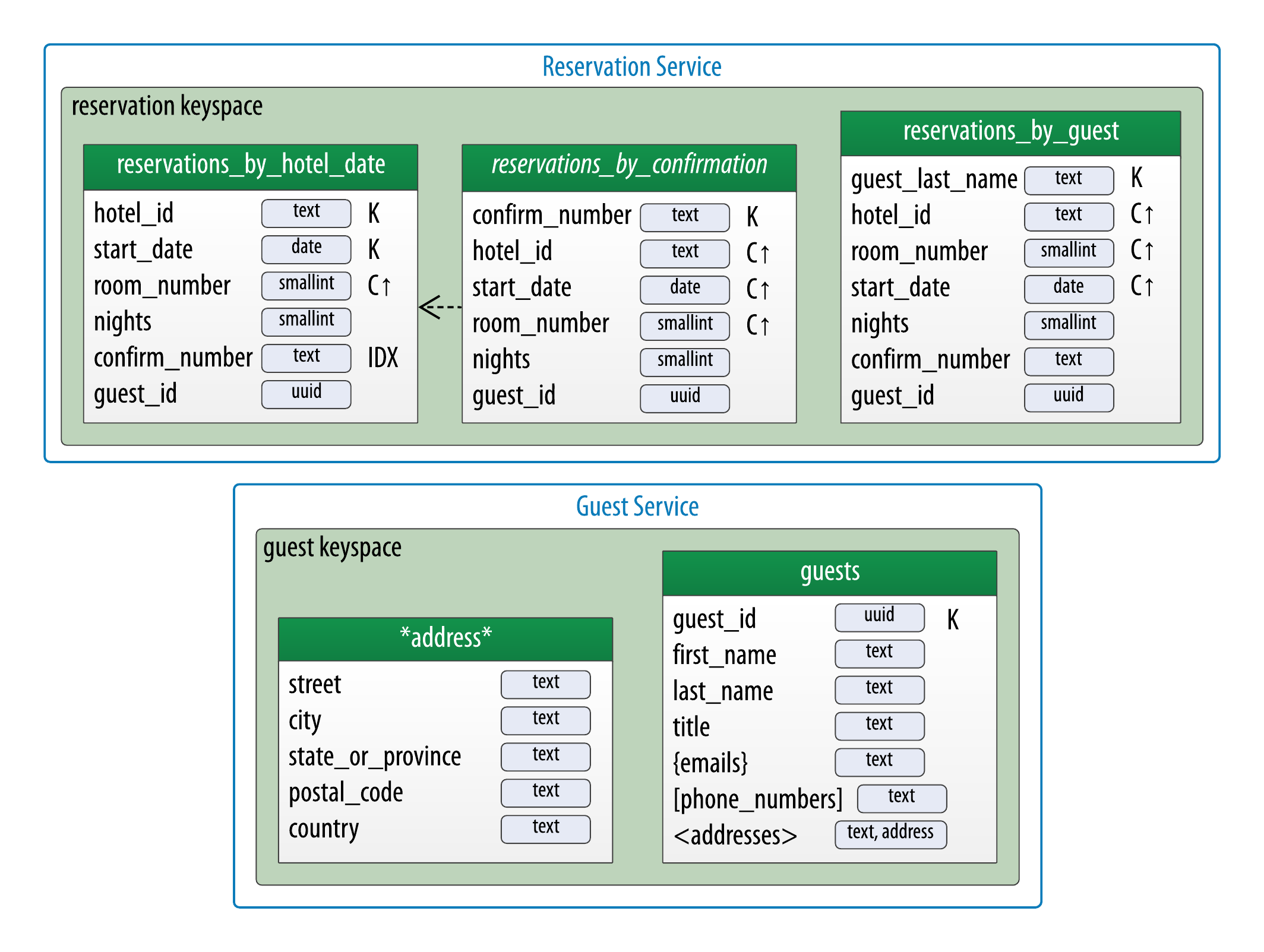
Figure 7-9. Revised Reservation Physical Model
Reservation Service: A Sample Microservice
So far, we’ve discussed how a microservice architecture is a natural fit for using Cassandra, identified candidate services for a hotel application, and considered how service design might influence our Cassandra data models. The final subject to examine is the design of individual microservices.
Design Choices for a Java Microservice
We’ll narrow our focus to the design of a single service: the Reservation Service. As discussed above, the Reservation Service will be responsible for reading and writing data using the tables in the reservation keyspace.
A candidate design for a Java implementation of the Reservation Service using popular libraries and frameworks is shown in Figure 7-10. THis implementation uses Apache Cassandra for its data storage via the DataStax Java Driver and the Spring Boot project for managing the service lifecycle. It exposes a RESTful API documented via Swagger.

Figure 7-10. Reservation Service Java Design
The Reservation Service Java implementation can be found on GitHub at: https://github.com/jeffreyscarpenter/reservation-service. The goal of this project is to provide a minimally functional implementation of a Java microservice using the DataStax Java Driver that can be used as a reference or starting point for other applications. We’ll be referencing this source code in Chapter 8 as we examine the functionality provided by the various DataStax drivers.
Deployment and Integration Considerations
As we proceed into implementation, there are a couple of factors we’ll want to consider related to how the service will be deployed and integrated with other services and supporting infrastructure.
Services, Keyspaces and Clusters
First, we’ll want to consider the relationship of services to keyspaces. A good rule of thumb is to use a keyspace per service to promote encapsulation. We’ll learn about Cassandra’s access control features in Chapter 14 that allow us to create a database user per keyspace, such that each service can be easily configured to have exclusive read and write access to all of the tables in its associated keyspace.
Next, we’ll want to consider whether a given service will have its own dedicated Cassandra cluster or share a cluster with other services. Figure 7-11 depicts a shared deployment in which Reservation and Inventory Services are using a shared cluster for data storage.
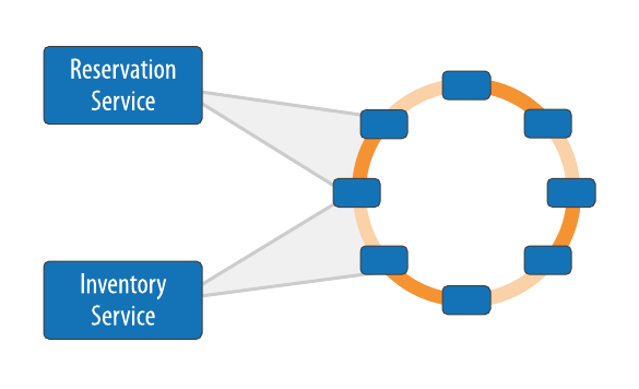
Figure 7-11. Service mapping to clusters
Companies that use both microservice architectures and Cassandra at large scale, such as Netflix, are known to use dedicated clusters per service. The decision of how many clusters to use will depend on the workload of each service. A flexible approach is to use a mix of shared and dedicated clusters, in which services that have lower demand share a cluster, while services with higher demand are deployed with their own dedicated cluster. Sharing a cluster across multiple services makes sense when the usage patterns of the services do not conflict.
Data Centers and Load Balancing
A second consideration is the selection of data centers where each service will be deployed. The corresponding cluster for a service should also have nodes in each data center where the service will be deployed, to enable the fastest possible access. Figure 7-12 shows a sample deployment across two data centers. The service instances should be made aware of the name of the local data center. The keyspace used by a service will need to be configured with a number of replicas to be stored per data center, assuming the NetworkTopoloyStrategy is the replication strategy in use.
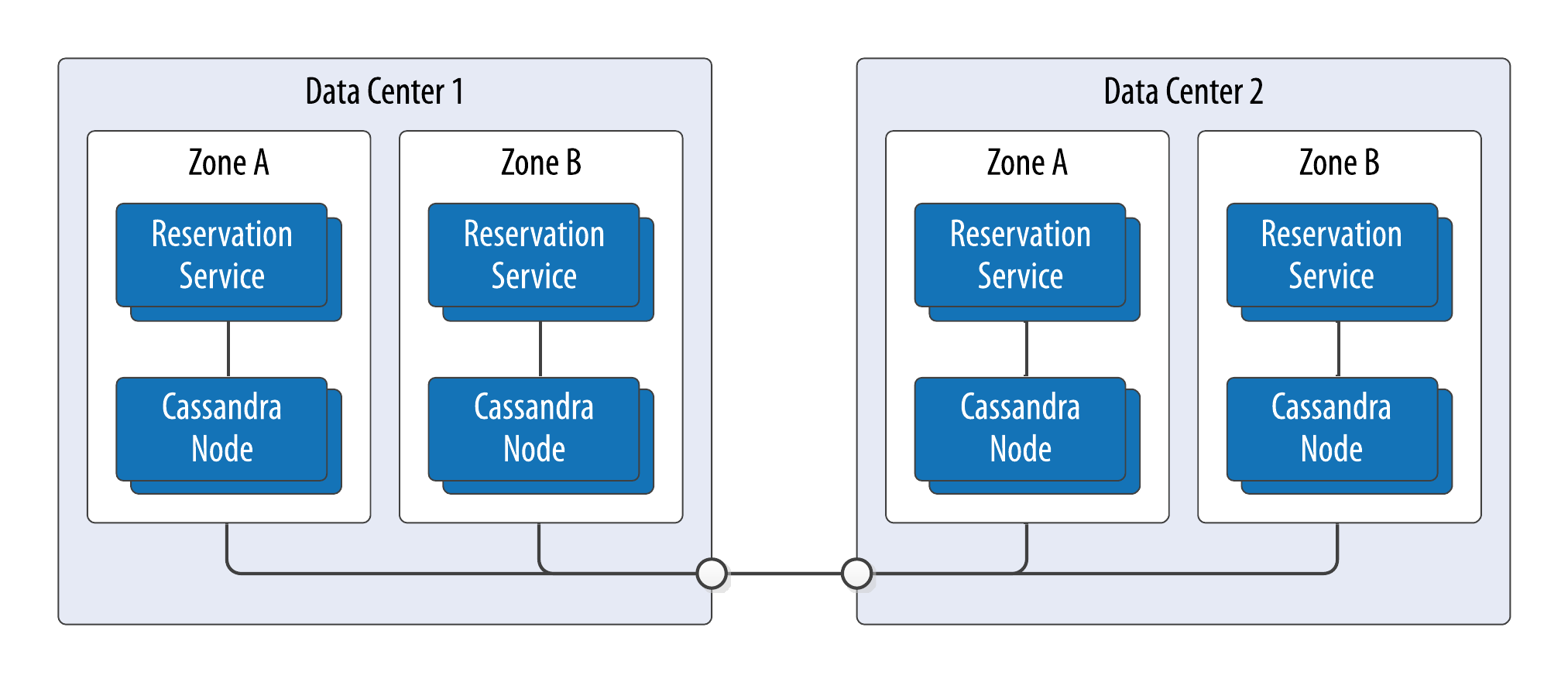
Figure 7-12. Multi-data center deployment
As you will learn in Chapter 8, most of these options such as keyspace names, database access credentials, and cluster topology can be externalized from application code into configuration files that can be more readily changed. Even so, it’s wise to begin thinking about these choices in the design phase.
Interactions Between Microservices
One question that arises when developing microservices that manage related types is how to maintain data consistency between the different types. If we insist on maintaining a strict ownership of data by different microservices, how can we maintain a consistency relationship for data types owned by different services? Cassandra does not provide us a mechanism to enforce transactions across table or keyspace boundaries. But this problem is not unique to Cassandra, since we’d have a similar design challenge whenever we need consistency between data types managed by different services, regardless of the backing store.
Let’s look at our hotel application for an example. Given that we’ve elected to have separate services to manage inventory and reservation data, how do we ensure that the inventory records are correctly updated when a customer makes a reservation? Two common approaches to this challenge are shown in Figure 7-13.
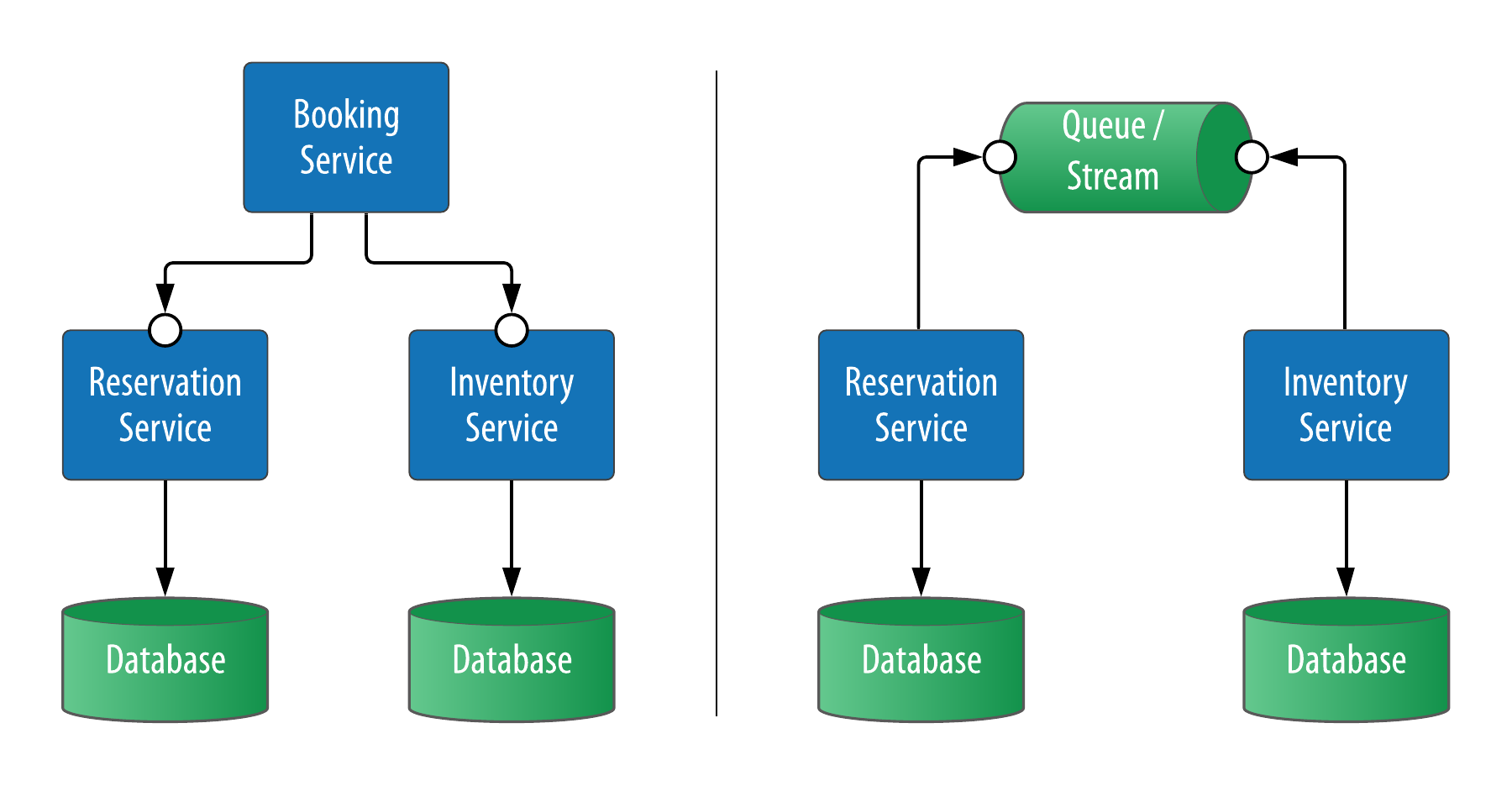
Figure 7-13. Service Integration Patterns
The approach on the left side is to create a Booking Service to help coordinate the changes to reservation and inventory data. This is an instance of a technique known as orchestration, often seen in architectures distinguish between so-called CRUD services (responsible for creating, reading, updating and deleting a specific data type) and services that implement business processes. In this example, the Reservation and Inventory Services are more CRUD services, while the Booking Service implements the business process of booking a reservation, reserving inventory and possibly other activities such as notifying the customer and hotel.
An alternative approach is depicted on the right side of the figure, in which a message queue or streaming platform such as Apache Kafka is used to create a stream of data change events which can be consumed asynchronously by other services and applications. For example, the Inventory Service might choose to subscribe to events related to reservations published by the Reservation Service in order to make corresponding adjustments to inventory. Because there is no central entity orchestrating these changes, this approach is instead known as choreography. We’ll examine integrating Cassandra with Kafka and other complementary technologies in more detail in Chapter 15.
It’s important to note that both orchestration and choreography can exhibit the tradeoffs between consistency, availability and partition tolerance that we discussed in Chapter 2 and will require careful planning to address error cases such as service and infrastructure failures. While a detailed treatment of these approaches including error handling scenarios is beyond our scope here, techniques and technologies are available to address error cases such as service failure and data inconsistency. These include:
-
Using a distributed transaction framework to coordinate changes across multiple services and databases. This can be a good approach when strong consistency is required. Scalar DB is an interesting library for implementing distributed ACID transactions that is built using Cassandra’s Lightweight Transactions as a locking primitive.
-
Using a distributed analytics tool such as Apache Spark to check data for consistency as a background processing task. This approach is useful as a backstop for catching data inconsistencies caused by software errors, in situations in which there is tolerance for temporary data inconsistencies.
-
A variant of the event-based choreography approach is to leverage the change data capture (CDC) feature of a database as the source of events, rather than relying on a service to reliably persist data to a database and then post an event. This approach is typically used to guarantee highly consistent interactions at the interface between applications, although it could be used between individual services.
Summary
In this chapter, we’ve looked at why Cassandra is a natural fit within a microservice style architecture and discussed how to ensure your architecture and data modeling processes can work together. We examined techniques for putting Cassandra based services in context of other data models. Now that we have examined the design of a particular microservice architecture, we’re ready to dive into the details of implementing applications using Cassandra.