Chapter 9. Writing and Reading Data
Now that you understand the data model and how to use a simple client, let’s dig deeper into the different kinds of queries you can perform in Cassandra to write and read data. We’ll also take a look behind the scenes to see how Cassandra handles your queries. Understanding these details will help you design queries that will perform well and provide the behavior you need.
As with the previous chapter, we’ve included code samples using the DataStax Java Driver to help illustrate how these concepts work in practice.
Writing
Let’s start by noting some basic properties of writing data to Cassandra. First, writing data is very fast in Cassandra, because its design does not require performing disk reads or seeks. The memtables and SSTables save Cassandra from having to perform these operations on writes, which slow down many databases. All writes in Cassandra are append-only.
Because of the database commit log and hinted handoff design, the database is always writable, and within a row, writes are always atomic.
Write Consistency Levels
Cassandra’s tuneable consistency levels mean that you can specify in your queries how much consistency you require on writes. A higher consistency level means that more replica nodes need to respond, indicating that the write has completed. Higher consistency levels also come with a reduction in availability, as more nodes must be operational for the write to succeed. The implications of using the different consistency levels on writes are shown in Table 9-1.
| Consistency level | Implication |
|---|---|
|
Ensure that the value is written to a minimum of one replica node before returning to the client, allowing hints to count as a write. |
|
Ensure that the value is written to the commit log and memtable of at least one, two, or three nodes before returning to the client. |
|
Similar to |
|
Ensure that the write was received by at least a majority of replicas (( |
|
Similar to |
|
Ensure that a |
|
Ensure that the number of nodes specified by |
The most notable consistency level for writes is the ANY level. This level means that the write is guaranteed to reach at least one node, but it allows a hint to count as a successful write. That is, if you perform a write operation and the node that the operation targets for that value is down, the server will make a note to itself, called a hint, which it will store until that node comes back up. Once the node is up, the server will detect this, look to see whether it has any writes that it saved for later in the form of a hint, and then write the value to the revived node. In many cases, the node that makes the hint actually isn’t the node that stores it; instead, it sends it off to one of the non-replica neighbors of the node that is down.
Using the consistency level of ONE on writes means that the write operation will be written to both the commit log and the memtable. That means that writes at ONE are durable, so this level is the minimum level to use to achieve fast performance and durability. If this node goes down immediately after the write operation, the value will have been written to the commit log, which can be replayed when the server is brought back up to ensure that it still has the value.
The Cassandra Write Path
The write path describes how data modification queries initiated by clients are processed, eventually resulting in the data being stored on disk. We’ll examine the write path in terms of both interactions between nodes and the internal process of storing data on an individual node. An overview of the write path interactions between nodes in a multi-data center cluster is shown in Figure 9-1.
The write path begins when a client initiates a write query to a Cassandra node which serves as the coordinator for this request. The coordinator node uses the partitioner to identify which nodes in the cluster are replicas, according to the replication factor for the keyspace. The coordinator node may itself be a replica, especially if the client is using a token-aware driver. If the coordinator knows that there are not enough replicas up to satisfy the requested consistency level, it returns an error immediately.
Next, the coordinator node sends simultaneous write requests to all replicas for the data being written. This ensures that all nodes will get the write as long as they are up. Nodes that are down will not have consistent data, but they will be repaired via one of the anti-entropy mechanisms: hinted handoff, read repair, or anti-entropy repair.

Figure 9-1. Interactions between nodes on the write path
If the cluster spans multiple data centers, the local coordinator node selects a remote coordinator in each of the other data centers to coordinate the write to the replicas in that data center. Each of the remote replicas responds directly to the original coordinator node.
The coordinator waits for the replicas to respond. Once a sufficient number of replicas have responded to satisfy the consistency level, the coordinator acknowledges the write to the client. If a replica doesn’t respond within the timeout, it is presumed to be down, and a hint is stored for the write. A hint does not count as successful replica write unless the consistency level ANY is used.
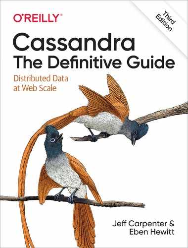
Figure 9-2 depicts the interactions that take place within each replica node to process a write request. These steps are common in databases that share the log-structured merge tree design we explored in Chapter 6.
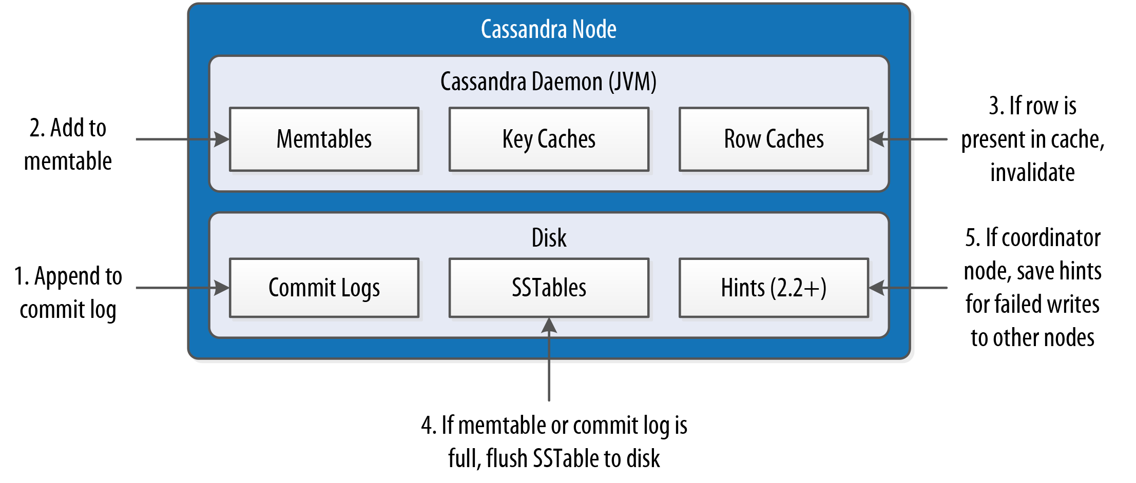
Figure 9-2. Interactions within a node on the write path
First, the replica node receives the write request and immediately writes the data to the commit log. Next, the replica node writes the data to a memtable. If row caching is used and the row is in the cache, the row is invalidated. We’ll discuss caching in more detail under the read path.
If the write causes either the commit log or memtable to pass its maximum thresholds, a flush is scheduled to run. We’ll learn how to tune these thresholds in Chapter 13.
At this point, the write is considered to have succeeded and the node can reply to the coordinator node or client.
After returning, the node executes a flush if one was scheduled. The contents of each memtable are stored as SSTables on disk and the commit log is cleared. After the flush completes, additional tasks are scheduled to check if compaction is needed and then a compaction is performed if necessary.
More Detail on the Write Path
Of course, this is a simple overview of the write path that doesn’t take into account variants such as counter modifications and materialized views. For example, writes to tables with materialized views are more complex because partitions must be locked while consensus is negotiated between replicas. Cassandra leverages logged batches internally in order to maintain materialized views.
Writing Files to Disk
Let’s examine a few more details on the files Cassandra writes to disk, including commit logs and SSTables.
Commit log files
Cassandra writes commit logs to the filesystem as binary files. The commit log files are found under the $CASSANDRA_HOME/data/commitlog directory.
Commit log files are named according to the pattern CommitLog-<version><timestamp>.log. For example: CommitLog-7-1566780133999.log. The version is an integer representing the commit log format. For example, the version for the 4.0 release is 7. You can find the versions in use by release in the org.apache.cassandra.db.commitlog.CommitLogDescriptor class.
SSTable files
When SSTables are written to the filesystem during a flush, there are actually several files that are written per SSTable. Let’s take a look at the $CASSANDRA_HOME/data/data directory to see how the files are organized on disk.
Forcing SSTables to Disk
If you’re following along with the exercises in this book on a real Cassandra node, you may want to execute the nodetool flush command at this point, as you may not have entered enough data yet for Cassandra to have flushed data to disk automatically. You’ll learn more about this command in Chapter 12.
Looking in the data directory, you’ll see a directory for each keyspace. These directories, in turn, contain a directory for each table, consisting of the table name plus a UUID. The purpose of the UUID is to distinguish between multiple schema versions, because the schema of a table can be altered over time.
Each of these directories contain SSTable files which contain the stored data. Here is an example directory path: hotel/hotels-3677bbb0155811e5899aa9fac1d00bce.
Each SSTable is represented by multiple files that share a common naming scheme. The files are named according to the pattern <version>-<generation>-<implementation>-<component>.db. The significance of the pattern is as follows:
-
The version is a two-character sequence representing the major/minor version of the SSTable format. For example, the version for the 4.0 release is na. You can learn more about various versions in the
org.apache.cassandra.io.sstable.Descriptorclass. -
The generation is an index number which is incremented every time a new SSTable is created for a table.
-
The implementation is a reference to the implementation of the
org.apache.cassandra.io.sstable.format.SSTableWriterinterface in use. As of the 4.0 release the value is “big”, which references the “Bigtable format” found in theorg.apache.cassandra.io.sstable.format.big.BigFormatclass.
Each SSTable is broken up into multiple files or components. These are the components as of the 3.0 release:
- Data.db
-
These are the files that store the actual data and are the only files that are preserved by Cassandra’s backup mechanisms, which you’ll learn about in Chapter 12.
- CompressionInfo.db
-
Provides metadata about the compression of the Data.db file.
- Digest.crc32
-
Contains a CRC 32 checksum for the *-Data.db file.
- Filter.db
-
Contains the bloom filter for this SSTable.
- Index.db
-
Provides row and column offsets within the corresponding *-Data.db file. The contents of this file are read into memory so that Cassandra knows exactly where to look when reading data files.
- Summary.db
-
A sample of the index for even faster reads.
- $Statistics.db
-
Stores statistics about the SSTable which are used by the
nodetool tablehistogramscommand. - $TOC.txt
-
Lists the file components for this SSTable.
Older releases support different versions and filenames. Releases prior to 2.2 prepend the keyspace and table name to each file, while 2.2 and later leave these out because they can be inferred from the directory name.
We’ll investigate some tools for working with SSTable files in Chapter 12.
Lightweight Transactions
As we’ve discussed previously in Chapter 1, Cassandra and many other NoSQL databases do not support transactions with full ACID semantics supported by relational databases. However, Cassandra does provide two mechanisms that offer some transactional behavior: lightweight transactions and batches.
Cassandra’s lightweight transaction (LWT) mechanism uses the Paxos algorithm described in Chapter 6. LWTs were introduced in the 2.0 release. LWTs support the following semantics:
-
On an
INSERT, adding theIF NOT EXISTSclause will ensure that you do not overwrite an existing row with the same primary key. This is frequently used in cases where uniqueness is important, such as managing user identity or accounts, or maintaining unique reservation records as you’ll see below. Alternatively, theIF EXISTSclause will only update the row with the provided primary key if it is already present in the database. This is effectively limiting Cassandra’s upsert behavior. -
On an
UPDATE, adding anIF <conditions>clause will perform a check of one or more provided conditions, where multiple conditions are separated by anAND. Each condition is a check against a column in aWHEREclause using operators including equality operators (=,!=), comparison operators (>,>=,<,⇐) and theINoperator. This is frequently used to make sure that a row has an expected value that cannot change before a write occurs. If a transaction fails because the existing values did not match the ones you expected, Cassandra will include the current values so you can decide whether to retry or abort without needing to make an extra request. This form of lightweight transaction is frequently used for managing inventory counts.
Let’s say you wanted to create a record for a new hotel, using the data model introduced in Chapter 5. You want to make sure that you’re not overwriting a reservation with the same confirmation number, so you add the IF NOT EXISTS syntax to your insert command:
cqlsh> INSERT INTO reservation.reservations_by_confirmation (confirmation_number, hotel_id, start_date, end_date, room_number, guest_id) VALUES (
  'RS2G0Z', 'NY456', '2020-06-08', '2020-06-10', 111, 1b4d86f4-ccff-4256-a63d-45c905df2677) IF NOT EXISTS;

 [applied]
-----------
      True
This command checks to see if there is a record with the partition key, which for this table consists of the confirmation_number. So let’s find out what happens when you execute this command a second time:
cqlsh> INSERT INTO reservation.reservations_by_confirmation (confirmation_number, hotel_id, start_date, end_date, room_number, guest_id) VALUES ('RS2G0Z', 'NY456', '2020-06-08', '2020-06-10', 111, 1b4d86f4-ccff-4256-a63d-45c905df2677) IF NOT EXISTS;

 [applied] | confirmation_number | end_date   | guest_id                             | hotel_id | room_number | start_date
-----------+---------------------+------------+--------------------------------------+----------+-------------+------------
     False |              RS2G0Z | 2020-06-10 | 1b4d86f4-ccff-4256-a63d-45c905df2677 |    NY456 |         111 | 2020-06-08
In this case, the transaction fails, because there is already a reservation with the number “RS2G0Z”, and cqlsh helpfully echoes back a row containing a failure indication and the values we tried to enter.
It works in a similar way for updates. For example, you might use the following statement to make sure you’re changing the end date for a reservation, but only if the previous value is the end date you expect:
cqlsh> UPDATE reservation.reservations_by_confirmation SET end_date='2020-06-12'
... WHERE confirmation_number='RS2G0Z' IF end_date='2020-06-10';

 [applied]
-----------
      True
Similar to what you saw with multiple INSERT statements, entering the same UPDATE statement again fails because the value has already been set. Because of Cassandra’s upsert model, the IF NOT EXISTS syntax available on INSERT and the IF x=y syntax on UPDATE represent the main semantic difference between these two operations.
Using Lightweight Transactions on Schema Creation
CQL also supports the use of the IF NOT EXISTS option on the creation of keyspaces and tables. This is especially useful if you are scripting multiple schema updates.
Let’s implement the reservation INSERT using the DataStax Java Driver. When executing a conditional statement the ResultSet will contain a single Row with a column named applied of type boolean. This tells whether the conditional statement was successful or not. You can also use the wasApplied() operation on the statement:
SimpleStatement reservationInsert = SimpleStatement.builder(
  "INSERT INTO reservations_by_confirmation (confirmation_number, hotel_id, start_date, end_date, room_number, guest_id) VALUES (?, ?, ?, ?, ?, ?)")
  .addPositionalValue("RS2G0Z")
  .addPositionalValue("NY456")
  .addPositionalValue("2020-06-08")
  .addPositionalValue("2020-06-10")
  .addPositionalValue(111)
  .addPositionalValue("1b4d86f4-ccff-4256-a63d-45c905df2677")
  <strong><code>.ifNotExists()</code></strong>
  .build();

ResultSet reservationInsertResult = session.execute(reservationInsert);

boolean wasApplied = reservationInsertResult.wasApplied());

if (wasApplied) {
  Row row = reservationInsertResult.one();
  row.getBool("applied");
}
This is a simple example using hardcoded values for readability rather than variables. You can find a working code sample for inserting reservation data using lightweight transactions on the lightweight-transaction-solution branch of the Reservation Service repository.
Conditional write statements can have a serial consistency level in addition to the regular consistency level. The serial consistency level determines the number of nodes that must reply in the Paxos phase of the write, when the participating nodes are negotiating about the proposed write. The two available options are shown in Table 9-2.
| Consistency level | Implication |
|---|---|
|
This is the default serial consistency level, indicating that a quorum of nodes must respond. |
|
Similar to |
The serial consistency level can apply on reads as well. If Cassandra detects that a query is reading data that is part of an uncommitted transaction, it commits the transaction as part of the read, according to the specified serial consistency level.
You can set a default serial consistency level for all statements in cqlsh using the SERIAL CONSISTENCY statement, or in the DataStax Java Driver using the serial-consistency configuration option. To override the configured level on an individual statement, use the Statement.setSerialConsistencyLevel() operation.
Batches
While lightweight transactions are limited to a single partition, Cassandra provides a batch mechanism that allows you to group modifications to multiple partitions into a single statement.
The semantics of the batch operation are as follows:
-
Only modification statements (
INSERT,UPDATE, orDELETE) may be included in a batch. -
Batches may be logged or unlogged, where logged batches have more safeguards. We’ll explain this in more detail below.
-
Batches are not a transaction mechanism, but you can include lightweight transaction statements in a batch. Multiple lightweight transactions in a batch must apply to the same partition.
-
Counter modifications are only allowed within a special form of batch known as a counter batch. A counter batch can only contain counter modifications.
Using a batch saves back and forth traffic between the client and the coordinator node, as the client is able to group multiple statements in a single query. However, the batch places additional work on the coordinator to orchestrate the execution of the various statements.
Cassandra’s batches are a good fit for use cases such as making multiple updates to a single partition, or keeping multiple tables in sync. A good example is making modifications to denormalized tables that store the same data for different access patterns.
Batches Aren’t for Bulk Loading
First time users often confuse batches for a way to get faster performance for bulk updates. This is definitely not the case—batches actually decrease performance and can cause garbage collection pressure. We’ll look at tools for bulk loading in Chapter 15.
In previous examples, you’ve inserted rows into the reservations_by_confirmation table, but remember that there is also a denormalized table design for reservations: reservations_by_hotel_date. Let’s use a batch to group those writes together.
You use the CQL BEGIN BATCH and APPLY BATCH keywords to surround the statements in your batch:
cqlsh>BEGIN BATCHINSERT INTO reservation.reservations_by_confirmation (confirmation_number, hotel_id, start_date, end_date, room_number, guest_id) VALUES ('RS2G0Z', 'NY456', '2020-06-08', '2020-06-10', 111, 1b4d86f4-ccff-4256-a63d-45c905df2677); INSERT INTO reservation.reservations_by_hotel_date (confirmation_number, hotel_id, start_date, end_date, room_number, guest_id) VALUES ('RS2G0Z', 'NY456', '2020-06-08', '2020-06-10', 111, 1b4d86f4-ccff-4256-a63d-45c905df2677);APPLY BATCH;
The DataStax Java driver supports batches through the com.datastax.oss.driver.api.core.cql.BatchStatement class. Here’s an example of what the same batch would look like in a Java client:
SimpleStatement reservationByConfirmationInsert = SimpleStatement.builder(
  "INSERT INTO reservations_by_confirmation (confirmation_number, hotel_id, start_date, end_date, room_number, guest_id) VALUES (?, ?, ?, ?, ?, ?)")
  .addPositionalValue("RS2G0Z")
  .addPositionalValue("NY456")
  .addPositionalValue("2020-06-08")
  .addPositionalValue("2020-06-10")
  .addPositionalValue(111)
  .addPositionalValue("1b4d86f4-ccff-4256-a63d-45c905df2677")
  .build();

SimpleStatement reservationByHotelDateInsert = SimpleStatement.builder(
  "INSERT INTO reservations_by_hotel_date (confirmation_number, hotel_id, start_date, end_date, room_number, guest_id) VALUES (?, ?, ?, ?, ?, ?)")
  .addPositionalValue("RS2G0Z")
  .addPositionalValue("NY456")
  .addPositionalValue("2020-06-08")
  .addPositionalValue("2020-06-10")
  .addPositionalValue(111)
  .addPositionalValue("1b4d86f4-ccff-4256-a63d-45c905df2677")
  .build();

BatchStatement reservationBatch = new BatchStatement();
reservationBatch.add(reservationByConfirmationInsert);
reservationBatch.add(reservationByHotelDateInsert);

cqlSession.execute(reservationBatch);
You can also create batches using a BatchStatementBuilder. You can find an example of working with BatchStatement on the batch-statement-solution branch of the Reservation Service repository.
Creating Counter Batches in DataStax Drivers
The DataStax drivers do not provide separate mechanisms for counter batches. Instead, you must simply remember to create batches that include only counter modifications or only non-counter modifications.
Logged batches are atomic—that is, if the batch is accepted, all of the statements in a batch will succeed eventually. This is why logged batches are sometimes referred to as atomic batches. Note that this is not the same definition of atomicity you might be used to if you have a relational database background. While all updates in a batch belonging to a given partition key are performed atomically, there is no guarantee across partitions. This means that modifications to different partitions may be read before the batch completes.
Here’s how a logged batch works under the covers: the coordinator sends a copy of the batch called a batchlog to two other nodes, where it is stored in the system.batchlog table. The coordinator then executes all of the statements in the batch, and deletes the batchlog from the other nodes after the statements are completed.
If the coordinator should fail to complete the batch, the other nodes have a copy in their batchlog and are therefore able to replay the batch. Each node checks its batchlog once a minute to see if there are any batches that should have completed. To give ample time for the coordinator to complete any in-progress batches, Cassandra uses a grace period from the timestamp on the batch statement equal to twice the value of the write_request_timeout_in_ms property. Any batches that are older than this grace period will be replayed and then deleted from the remaining node. The second batchlog node provides an additional layer of redundancy, ensuring high reliability of the batch mechanism.
In an unlogged batch, the steps involving the batchlog are skipped, allowing the write to complete more quickly. Users who are trying to rapidly insert a lot of data are often tempted to use unlogged batches. The tradeoff you’ll want to consider is that there is no guarantee that all of the writes to different partitions will complete successfully, which could leave the database in an inconsistent state. This risk does not exist when a batch contains mutations to a single partition. For this reason, if you request a logged batch with mutations to a single partition, Cassandra actually executes it as an unlogged batch to give you an extra boost of speed.
Another factor you should consider is the size of batches, measured in terms of the total data size in bytes rather than a specific number of statements. Cassandra enforces limits on the size of batch statements to prevent them from becoming arbitrarily large and impacting the performance and stability of the cluster. The cassandra.yaml file contains two properties that control how this works: the batch_size_warn_threshold_in_kb property defines the level at which a node will log at the WARN log level that it has received a large batch, while any batch exceeding the value set batch_size_fail_threshold_in_kb will be rejected and result in error notification to the client. The batch size is measured in terms of the length of the CQL query statement. The warning threshold defaults to 5KB, while the fail threshold defaults to 50KB.
Reading
There are a few basic properties of Cassandra’s read capability that are worth noting. First, it’s easy to read data because clients can connect to any node in the cluster to perform reads, without having to know whether a particular node acts as a replica for that data. If a client connects to a node that doesn’t have the data it’s trying to read, the node it’s connected to will act as coordinator node to read the data from a node that does have it, identified by token ranges.
In Cassandra, reads are generally slower than writes due to file I/O from reading SSTables. To fulfill read operations, Cassandra typically has to perform seeks, but you may be able to keep more data in memory by adding nodes, using compute instances with more memory, and using Cassandra’s caches. Cassandra also has to wait for responses synchronously on reads (based on consistency level and replication factor), and then perform read repairs as necessary.
Read Consistency Levels
The consistency levels for read operations are similar to the write consistency levels, but the way they are handled behind the scenes is slightly different. A higher consistency level means that more nodes need to respond to the query, giving you more assurance that the values present on each replica are the same. If two nodes respond with different timestamps, the newest value wins, and that’s what will be returned to the client. In the background, Cassandra will then perform what’s called a read repair: it takes notice of the fact that one or more replicas responded to a query with an outdated value, and updates those replicas with the most current value so that they are all consistent.
The possible consistency levels, and the implications of specifying each one for read queries, are shown in Table 9-3.
| Consistency level | Implication |
|---|---|
|
Immediately return the record held by the first node(s) that respond to the query. A background thread is created to check that record against the same record on other replicas. If any are out of date, a read repair is then performed to sync them all to the most recent value. |
|
Similar to |
|
Query all nodes. Once a majority of replicas (( |
|
Similar to |
|
Ensure that a |
|
Query all nodes. Wait for all nodes to respond, and return to the client the record with the most recent timestamp. Then, if necessary, perform a read repair in the background. If any nodes fail to respond, fail the read operation. |
As you can see from the table, the ANY consistency level is not supported for read operations. Notice that the implication of consistency level ONE is that the first node to respond to the read operation is the value that the client will get—even if it is out of date. The read repair operation is performed after the record is returned, so any subsequent reads will all have a consistent value, regardless of the responding node.
Another item worth noting is in the case of consistency level ALL. If you specify ALL, then you’re saying that you require all replicas to respond, so if any node with that record is down or otherwise fails to respond before the timeout, the read operation fails. A node is considered unresponsive if it does not respond to a query before the value specified by read_request_timeout_in_ms in the configuration file. The default is 5 seconds.
The Cassandra Read Path
Now let’s take a look at what happens when a client requests data. This is known as the read path. We’ll describe the read path from the perspective of a query for a single partition key, starting with the interactions between nodes shown in Figure 9-3.
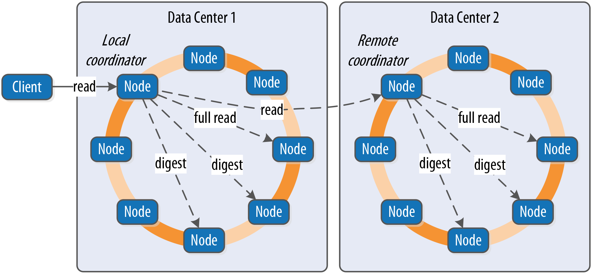
Figure 9-3. Interactions between nodes on the read path
The read path begins when a client initiates a read query to the coordinator node. As on the write path, the coordinator uses the partitioner to determine the replicas and checks that there are enough replicas up to satisfy the requested consistency level. Another similarity to the write path is that a remote coordinator is selected per data center for any read queries that involve multiple data centers.
If the coordinator is not itself a replica, the coordinator then sends a read request to the fastest replica, as determined by the dynamic snitch. The coordinator node also sends a digest request to the other replicas. A digest request is similar to a standard read request, except the replicas return a digest, or hash, of the requested data.
The coordinator calculates the digest hash for data returned from the fastest replica and compares it to the digests returned from the other replicas. If the digests are consistent, and the desired consistency level has been met, then the data from the fastest replica can be returned. If the digests are not consistent, then the coordinator must perform a read repair, as discussed in the following section.
Figure 9-4 shows the interactions that take place within each replica node to process read requests.
Figure 9-4. Interactions within a node on the read path
When the replica node receives the read request, it first checks the row cache. If the row cache contains the data, it can be returned immediately. The row cache helps speed read performance for rows that are accessed frequently. We’ll discuss the pros and cons of row caching in Chapter 13.
If the data is not in the row cache, the replica node searches for the data in memtables and SSTables. There is only a single memtable for a given table, so that part of the search is straightforward. However, there are potentially many physical SSTables for a single Cassandra table, each of which may contain a portion of the requested data.
Cassandra implements several features to optimize the SSTable search: key caching, Bloom filters, SSTable indexes, and summary indexes.
The first step in searching SSTables on disk is to use a Bloom filter to determine whether requested partition does not exist in a given SSTable, which would make it unnecessary to search that SSTable.
If the SSTable passes the Bloom filter, Cassandra checks the key cache to see if it contains the offset of the partition key in the SSTable. The key cache is implemented as a map structure in which the keys are a combination of the SSTable file descriptor and partition key, and the values are offset locations into SSTable files. The key cache helps to eliminate seeks within SSTable files for frequently accessed data, because the data can be read directly.
If the offset is not obtained from the key cache, Cassandra uses a two-level index stored on disk in order to locate the offset. The first level index is the partition summary, which is used to obtain an offset for searching for the partition key within the second level index, the partition index. The partition index is where the offset into the SSTable for the partition key is stored.
If the offset for the partition key is found, Cassandra accesses the SSTable at the specified offset and starts reading data.
Once data has been obtained from all of the SSTables, Cassandra merges the SSTable data and memtable data by selecting the value with the latest timestamp for each requested column. Any tombstones encountered are ignored.
Finally, the merged data can be added to the row cache (if enabled) and returned to the client or coordinator node. A digest request is handled in much the same way as a regular read request, with the additional step that a digest is calculated on the result data and returned instead of the data itself.
Read Repair
Here’s how read repair works: the coordinator makes a full read request from all of the replica nodes. The coordinator node merges the data by selecting a value for each requested column. It compares the values returned from the replicas and returns the value that has the latest timestamp. If Cassandra finds different values stored with the same timestamp, it will compare the values lexicographically and choose the one that has the greater value. This case should be exceedingly rare. The merged data is the value that is returned to the client.
Asynchronously, the coordinator identifies any replicas that return obsolete data and issues a read-repair request to each of these replicas to update their data based on the merged data.
The read repair may be performed either before or after the return to the client. If you are using one of the two stronger consistency levels (QUORUM or ALL), then the read repair happens before data is returned to the client. If the client specifies a weak consistency level (such as ONE), then the read repair is optionally performed in the background after returning to the client. The percentage of reads that result in background repairs for a given table is determined by the read_repair_chance and dc_local_read_repair_chance options for the table.
Range Queries, Ordering and Filtering
So far your read queries have been confined to very simple examples. Let’s take a look at more of the options that Cassandra provides on the SELECT command, such as the WHERE and ORDER BY clauses.
First, let’s examine how to use the WHERE clause that Cassandra provides for reading ranges of data within a partition, sometimes called slices.
In order to do a range query, however, it will help to have some data to work with. Although you don’t have a lot of data yet, you can quickly get some by using cqlsh to load some sample reservation data into your cluster. We’ll look at more advanced bulk loading options in Chapter 15.
You can access a simple .csv file in the GitHub repository for this book. The reservations.csv file contains a month’s worth of inventory for two small hotels with five rooms each. Let’s load the data into the cluster:
cqlsh:hotel> COPY available_rooms_by_hotel_date FROM
  'available_rooms.csv' WITH HEADER=true;

310 rows imported in 0.789 seconds.
If you do a quick query to read some of this data, you’ll find that you have data for two hotels: “AZ123” and “NY229”.
Now let’s consider how to support the query labeled “Q4. Find an available room in a given date range” in Chapter 5. Remember that the available_rooms_by_hotel_date table was designed to support this query, with the primary key:
PRIMARY KEY (hotel_id, date, room_number)
This means that the hotel_id is the partition key, while date and room_number are clustering columns.
Here’s a CQL statement that allows you to search for hotel rooms for a specific hotel and date range:
cqlsh:hotel> SELECT * FROM available_rooms_by_hotel_date
  WHERE hotel_id='AZ123' and date>'2016-01-05' and date<'2016-01-12';

 hotel_id | date       | room_number | is_available
----------+------------+-------------+--------------
    AZ123 | 2016-01-06 |         101 |         True
    AZ123 | 2016-01-06 |         102 |         True
    AZ123 | 2016-01-06 |         103 |         True
    AZ123 | 2016-01-06 |         104 |         True
    AZ123 | 2016-01-06 |         105 |         True
...
(60 rows)
Note that this query involves the partition key hotel_id and a range of values representing the start and end of your search over the clustering key date.
If you wanted to try to find the records for room number 101 at hotel AZ123, you might attempt a query like the following:
cqlsh:hotel> SELECT * FROM available_rooms_by_hotel_date
  WHERE hotel_id='AZ123' and room_number=101;
InvalidRequest: code=2200 [Invalid query] message="PRIMARY KEY column
  "room_number" cannot be restricted as preceding column "date" is not
  restricted"
As you can see, this query results in an error, because you have attempted to restrict the value of the second clustering key while not limiting the value of the first clustering key.
The syntax of the WHERE clause involves two rules. First, all elements of the partition key must be identified. Second, a given clustering key may only be restricted if all previous clustering keys are restricted.
These restrictions are based on how Cassandra stores data on disk, which is based on the clustering columns and sort order specified on the CREATE TABLE command. The conditions on the clustering column are restricted to those that allow Cassandra to select a contiguous ordering of rows.
The exception to this rule is the ALLOW FILTERING keyword, which allows you to omit a partition key element. For example, you can search the room status across multiple hotels for rooms on a specific date with this query:
cqlsh:hotel> SELECT * FROM available_rooms_by_hotel_date
  WHERE date='2016-01-25' ALLOW FILTERING;

 hotel_id | date       | room_number | is_available
----------+------------+-------------+--------------
    AZ123 | 2016-01-25 |         101 |         True
    AZ123 | 2016-01-25 |         102 |         True
    AZ123 | 2016-01-25 |         103 |         True
    AZ123 | 2016-01-25 |         104 |         True
    AZ123 | 2016-01-25 |         105 |         True
    NY229 | 2016-01-25 |         101 |         True
    NY229 | 2016-01-25 |         102 |         True
    NY229 | 2016-01-25 |         103 |         True
    NY229 | 2016-01-25 |         104 |         True
    NY229 | 2016-01-25 |         105 |         True

(10 rows)
Usage of ALLOW FILTERING is not recommended, however, as it has the potential to result in very expensive queries. If you find yourself needing such a query, you will want to revisit your data model to make sure you have designed tables that support your queries.
The IN clause can be used to test equality with multiple possible values for a column. For example, you could use the following to find inventory on two dates a week apart with the command:
cqlsh:hotel> SELECT * FROM available_rooms_by_hotel_date
  WHERE hotel_id='AZ123' AND date IN ('2016-01-05', '2016-01-12');
Note that using the IN clause to specify multiple clustering column values can result in slower performance on queries, as the specified column values may correspond to non-contiguous areas within the row.
Similarly, if you use the IN clause to specify multiple partitions, that would cause the coordinator node to have to talk to a greater number of nodes to support your query. In such a case, you might consider kicking off separate requests for the different partitions in parallel threads in your application so that the driver can directly contact a replica as the coordinator for each query.
Finally, the SELECT command allows you to override the sort order which has been specified on the columns when you created the table. For example, you could obtain the rooms in descending order by date for any of your previous queries using the ORDER BY syntax:
cqlsh:hotel> SELECT * FROM available_rooms_by_hotel_date
  WHERE hotel_id='AZ123' and date>'2016-01-05' and date<'2016-01-12'
  ORDER BY date DESC;
More on the WHERE clause
The DataStax Blog post “A deep look at the CQL WHERE clause” provides additional advice and examples on how to use the various options available on the WHERE clause.
Paging
In early releases of Cassandra, clients had to make sure to carefully limit the amount of data requested at a time. For a large result set, it is possible to overwhelm both nodes and clients even to the point of running out of memory.
Thankfully, Cassandra provides a paging mechanism that allows retrieval of result sets incrementally. A simple example of this is shown by use of the CQL keyword LIMIT. For example, the following command will return no more than 100 hotels:
cqlsh> SELECT * FROM reservation.reservations_by_hotel_date LIMIT 100;
Of course, the limitation of the LIMIT keyword (pun intended) is that there’s no way to obtain additional pages containing the additional rows beyond the requested quantity.
The 2.0 release of Cassandra introduced a feature known as automatic paging. Automatic paging allows clients to request a subset of the data that would be returned by a query. The server breaks the result into pages that are returned as the client requests them.
You can view paging status in cqlsh via the PAGING command. The following output shows a sequence of checking paging status, changing the fetch size (page size), and disabling paging:
cqlsh> PAGING;
Query paging is currently enabled. Use PAGING OFF to disable
Page size: 100
cqlsh> PAGING 1000;
Page size: 1000
cqlsh> PAGING OFF;
Disabled Query paging.
cqlsh> PAGING ON;
Now Query paging is enabled
Now let’s see how paging works in the DataStax Java Driver. You can set a default fetch size globally for a CqlSession instance using the basic.request.page-size parameter, which defaults to 5000. The page size can also be set on an individual statement, overriding the default value:
Statement statement = SimpleStatement.builder("...").build();
statement.setPageSize(2000);
The page size is not necessarily exact; the driver might return slightly more or slightly fewer rows than requested. The driver handles automatic paging on your behalf, allowing you to iterate over a ResultSet without requiring knowledge of the paging mechanism. For example, consider the following code sample for iterating over a query for hotels:
SimpleStatement reservationsByHotelDateSelect = SimpleStatement.builder(
  "SELECT * FROM reservations_by_hotel_date").build();
ResultSet resultSet = cqlSession.execute(reservationsByHotelDateSelect);

for (Row row : resultSet) {
  // process the row
}
What happens behind the scenes is as follows: when your application invokes the cqlSession.execute() operation, the driver performs your query to Cassandra, requesting the first page of results. Your application iterates over the results as shown in the for loop, and when the driver detects that there are no more items remaining on the current page, it requests the next page.
It is possible that the small pause of requesting the next page would affect the performance and user experience of your application, so the ResultSet provides additional operations that allow more fine grained control over paging. Here’s an example of how you could extend your application to do some pre-fetching of rows:
for (Row row : resultSet) {
  if (resultSet.getAvailableWithoutFetching() < 100 &&
      !resultSet.isFullyFetched())
        resultSet.fetchMoreResults();
  // process the row
}
This additional statement checks to see if there are less than 100 rows remaining on the current page using getAvailableWithoutFetching(). If there is another page to be retrieved, which you determine by checking isFullyFetched(), you initiate an asynchronous call to obtain the extra rows via fetchMoreResults().
The driver also exposes the ability to access the paging state more directly so it can be saved and reused later. This could be useful if your application is a stateless web service that doesn’t sustain a session across multiple invocations.
You can access the paging state through the ExecutionInfo of the ResultSet, which provides the state as an opaque array of bytes contained in a java.nio.ByteBuffer:
ByteBuffer nextPage = resultSet.getExecutionInfo().getPagingState();
You can then save this state within your application, or return it to clients. The paging state can be converted to a string using toString(), or a byte array using array().
Note that in either string or byte array form, the state is not something you should try to manipulate or reuse with a different statement. Doing so could result in an exception.
To resume a query from a given paging state, you set it on the Statement:
SimpleStatement reservationsByHotelDateSelect = SimpleStatement.builder(
  "SELECT * FROM reservation.reservations_by_hotel_date").build();
reservationsByHotelDateSelect.setPagingState(pagingState);
Deleting
Deleting data is not the same in Cassandra as it is in a relational database. In an RDBMS, you simply issue a delete statement that identifies the row or rows you want to delete. In Cassandra, a delete does not actually remove the data immediately. There’s a simple reason for this: Cassandra’s durable, eventually consistent, distributed design. If Cassandra had a traditional design for deletes, any nodes that were down at the time of a delete would not receive the delete. Once one of these nodes came back online, it would mistakenly think that all of the nodes that had received the delete had actually missed a write (the data that it still has because it missed the delete), and it would start repairing all of the other nodes. So Cassandra needs a more sophisticated mechanism to support deletes. That mechanism is called a tombstone.
A tombstone is a special marker issued in a delete that overwrites the deleted values, acting as a placeholder. If any replica did not receive the delete operation, the tombstone can later be propagated to those replicas when they are available again. The net effect of this design is that your data store will not immediately shrink in size following a delete. Each node keeps track of the age of all its tombstones. Once they reach the age as configured in gc_grace_seconds (which is 10 days by default), then a compaction is run, the tombstones are garbage-collected, and the corresponding disk space is recovered.
Because SSTables are immutable, the data is not deleted from the SSTable. On compaction, tombstones are accounted for, merged data is sorted, a new index is created over the sorted data, and the freshly merged, sorted, and indexed data is written to a single new file. The assumption is that 10 days is plenty of time for you to bring a failed node back online before compaction runs. If you feel comfortable doing so, you can reduce that grace period to reclaim disk space more quickly.
You’ve previously used the CQL DELETE command in Chapter 4. Here’s what a simple delete of an entire row looks like using the DataStax Java Driver:
SimpleStatement reservationByConfirmationDelete = SimpleStatement.builder(
  "DELETE * FROM reservation.reservations_by_confirmation WHERE confirmation_number=?")
  .addPositionalValue("RS2G0Z")
  .build();

cqlSession.execute(reservationByConfirmationDelete);
You can also delete data using PreparedStatements, the QueryBuilder, and the Mapper. Here is an example of deleting an entire row using the QueryBuilder:
import static com.datastax.oss.driver.api.querybuilder.QueryBuilder.*;

SimpleStatement reservationByConfirmationDelete = deleteFrom("reservations", "reservations_by_confirmation")
   .whereColumn("confirmation_number").isEqualTo("RS2G0Z")
   .build();

cqlSession.execute(reservationByConfirmationDelete);
Because a delete is a form of write, the consistency levels available for deletes are the same as those listed for writes.
Cassandra allows you to delete data at multiple levels of granularity. You can:
-
delete items from a collection (
set,list, ormap), as you learned in Chapter 4 -
delete non-primary key columns by identifying them by name in your
DELETEquery -
delete entire rows as shown above
-
delete ranges of rows using the same
WHEREclauses as with theSELECTcommand -
delete an entire partition
Because of how Cassandra tracks deletions, Each of these operations will result in a single tombstone. The more data you are able to delete in a single command, the fewer tombstones you will have. If your application generates a large number of tombstones, Cassandra’s read performance can begin to be impacted by having to traverse over these tombstones as it reads SSTable files. You’ll learn in Chapter 11 how to detect this issue, but it’s also wise to try to avoid it to begin with.
Here are a few techniques to help minimize the impact of tombstones on your cluster:
-
Avoid writing
NULLvalues into your tables, as these are interpreted as deletes. This can happen in cases where an unset attribute on a user interface or API is interpreted as aNULLvalue as it moves down through your application stack. While this is relatively simple to police in your own application code, mapping frameworks such as Spring Data Cassandra or the DataStax Java Driver’s Mapper can tend to abstract this behavior, which can lead to the generation of many tombstones without your knowledge. Make sure you investigate and properly configure the null-handling behavior you expect when using frameworks that abstract CQL queries. -
Delete data at the largest granularity you can, ideally entire partitions at once. This will minimize the number of tombstones you create. Alain Rodriguez’s blog post About Tombstones and Deletes in Cassandra explains this strategy in more depth.
-
Use Cassandra’s time-to-live (TTL) feature when inserting data, which allows Cassandra to expire data automatically on your behalf without generating tombstones.
-
For tables that implement a time-series pattern, consider using the
TimeWindowCompactionStrategy, which allows Cassandra to drop entire SSTable files at once. We’ll discuss this strategy further in Chapter 13.
Summary
In this chapter, you saw how to read, write, and delete data using both cqlsh and client drivers. You also took a peek behind the scenes to learn how Cassandra implements these operations, which should help you to make more informed decisions as you design, implement, deploy and maintain applications using Cassandra.