Creating a Cluster

The cassandra.yaml file is the primary configuration file for a Cassandra node, and where you specify the configuration values that define a cluster. You can find this file in the conf directory under your Cassandra installation.

The key values in configuring a cluster are the cluster name, the partitioner, the snitch, and the seed nodes. The cluster name, partitioner, and snitch must be the same in all of the nodes participating in the cluster. The seed nodes are not strictly required to be exactly the same for every node across the cluster, but it is a good idea to have a common set of seeds per data center; we’ll discuss configuration best practices momentarily.

Cassandra clusters are given names in order to prevent machines in one cluster from joining another that you don’t want them to be a part of. The name of the default cluster in the cassandra.yaml file is Test Cluster. You can change the name of the cluster by updating the cluster_name property—just make sure that you have done this on all nodes that you want to participate in this cluster.

Let’s try creating a cluster using ccm for use with the Reservation Service we’ve discussed in previous chapters (some of the output has been reduced for brevity):

$ ccm create -v 4.0.0 -n 3 reservation_cluster --vnodes
 ...
Current cluster is now: reservation_cluster

This command creates a cluster based on the version of Cassandra you select—in this case, 4.0.0. The cluster is named my_cluster and has three nodes. You must specify explicitly when youwant to use virtual nodes, because ccm defaults to creating single token nodes. ccm designates your cluster as the current cluster that will be used for subsequent commands. You’ll notice that it downloads the source for the version requested to run and compiles it. This is because it needs to make minor modifications to the Cassandra source in order to support running multiple nodes on a single machine. You could also have used the copy of the source downloaded in Chapter 3. If you’d like to investigate additional options for creating a cluster, run the command ccm create -h.

Once you’ve created the cluster, you’ll see it is the only cluster in your list of clusters (and marked as the currently selected cluster with an asterisk), and you can learn about its status:

$ ccm list
 *reservation_cluster

$ ccm status
Cluster: 'reservation_cluster'
---------------------
node1: DOWN (Not initialized)
node3: DOWN (Not initialized)
node2: DOWN (Not initialized)

At this point, none of the nodes have been initialized. Start your cluster and then check the status again:

$ ccm start

$ ccm status
Cluster: 'reservation_cluster'
---------------------
node1: UP
node3: UP
node2: UP

This is the equivalent of starting each individual node using the bin/cassandra script. To dig deeper on the status of an individual node, enter the following command:

$ ccm node1 status

Datacenter: datacenter1
=======================
Status=Up/Down
|/ State=Normal/Leaving/Joining/Moving
--  Address    Load        Tokens  Owns (effective)  Host ID       Rack
UN  127.0.0.1  115.13 KiB  256     67.5%             9019859a-...  rack1
UN  127.0.0.2  115.14 KiB  256     63.3%             5650bfa0-...  rack1
UN  127.0.0.3  115.13 KiB  256     69.2%             158a78c2-...  rack1

This is equivalent to running the command nodetool status on the individual node. The output shows that all of the nodes are up and reporting normal status (UN means “up normal”). Each of the nodes has 256 tokens and a very small amount of metadata, since you haven’t inserted any data yet. (We’ve shortened the Host ID somewhat for brevity.)

You run the nodetool ring command in order to get a list of the tokens owned by each node. To do this in ccm, enter the command:

$ ccm node1 ring

Datacenter: datacenter1
==========
Address    Rack        Status State   ...  Token
                                           9171899284504323785
127.0.0.1  rack1       Up     Normal  ...  -9181802192617819638
127.0.0.2  rack1       Up     Normal  ...  -9119747148344833344
127.0.0.2  rack1       Up     Normal  ...  -9114111430148268761
127.0.0.3  rack1       Up     Normal  ...  -9093245859094984745
127.0.0.2  rack1       Up     Normal  ...  -9093095684198819851

The command requires us to specify a node. This doesn’t affect the output; it just indicates what node nodetool is connecting to in order to get the ring information. As you can see, the tokens are allocated randomly across the three nodes. (As before, we’ve abbreviated the output and omitted the Owns and Load columns for brevity.)

Adding Nodes to a Cluster

Now that you understand what goes into configuring each node of a Cassandra cluster, you’re ready to learn how to add nodes. As we’ve already discussed, to add a new node manually, you need to configure the cassandra.yaml file for the new node to set the seed nodes, partitioner, snitch, and network ports. If you’ve elected to create single token nodes, you’ll also need to calculate the token range for the new node and make adjustments to the ranges of other nodes.

If you’re using ccm, the process of adding a new node is quite simple. Run the following command:

$ ccm add node4 -i 127.0.0.4 -j 7400

This creates a new node, node4, with another loopback address and JMX port set to 7400. To see additional options for this command you can type ccm add –h. Now that you’ve added a node, check the status of your cluster:

$ ccm status
Cluster: 'reservation_cluster'
---------------------
node1: UP
node3: UP
node2: UP
node4: DOWN (Not initialized)

The new node has been added but has not been started yet. If you run the nodetool ring command again, you’ll see that no changes have been made to the tokens. Now you’re ready to start the new node by typing ccm node4 start (after double-checking that the additional loopback address is enabled). If you run the nodetool ring command once more, you’ll see output similar to the following:

Datacenter: datacenter1
==========
Address    Rack        Status  State   ...  Token
                                            9218701579919475223
127.0.0.1  rack1       Up      Normal  ...  −9211073930147845649
127.0.0.4  rack1       Up      Normal  ...  −9190530381068170163
...

If you compare this with the previous output, you’ll notice a couple of things. First, the tokens have been reallocated across all of the nodes, including the new node. Second, the token values have changed, representing smaller ranges. In order to give your new node its 256 tokens (num_tokens), there are now 1,024 total tokens in the cluster.

You can observe what it looks like to other nodes when node4 starts up by examining the log file. On a standalone node, you might look at the system.log file in /var/log/cassandra (or $CASSANDRA_HOME/logs), depending on your configuration. ccm provides a handy command to examine the log files from any node. Look at the log for node1 using the command: ccm node1 showlog. This brings up a view similar to the standard unix more command that allows us to page through or search the log file contents. Searching for gossip-related statements in the log file near the end (for example, by typing /127.0.0.4), you’ll find something like this:

INFO  [GossipStage:1] 2019-11-27 15:40:51,176 Gossiper.java:1222 -
  Node 127.0.0.4:7000 is now part of the cluster
INFO  [GossipStage:1] 2019-11-27 15:40:51,203 TokenMetadata.java:490 -
  Updating topology for 127.0.0.4:7000
INFO  [GossipStage:1] 2019-11-27 15:40:51,206 StorageService.java:2524 -
  Node 127.0.0.4:7000 state jump to NORMAL
INFO  [GossipStage:1] 2019-11-27 15:40:51,213 Gossiper.java:1180 -
  InetAddress 127.0.0.4:7000 is now UP

These statements show node1 successfully gossiping with node4 and that node4 is considered up and part of the cluster. At this point, the bootstrapping process begins to allocate tokens to node4 and stream any data associated with those tokens to node4.

Dynamic Ring Participation

Nodes in a Cassandra cluster can be brought down and back up without disrupting the rest of the cluster (assuming a reasonable replication factor and consistency level). Say that you’ve started a two-node cluster, as described in “Creating a Cluster”. You can cause an error to occur that will take down one of the nodes, and then make sure that the rest of the cluster is still OK.

You can simulate this situation by taking one of the nodes down using the ccm stop command. We can run the ccm status to verify the node is down, and then check a log file as we did earlier via the ccm showlog command. If you stop node4, and examine the log file for another node, you’ll see something like the following:

INFO  [GossipStage:1] 2019-11-27 15:44:09,564 Gossiper.java:1198 -
  InetAddress 127.0.0.4:7000 is now DOWN

Now bring node4 back up and recheck the logs at another node. Sure enough, Cassandra has automatically detected that the other participant has returned to the cluster and is again open for business:

INFO  [GossipStage:1] 2019-11-27 15:45:34,579 Gossiper.java:1220 -
  Node 127.0.0.4:7000 has restarted, now UP

The state jump to normal for node4 indicates that it’s part of the cluster again. As a final check, we run the status command again:

$ ccm status
Cluster: 'reservation_cluster'
---------------------
node1: UP
node2: UP
node3: UP
node4: UP

As you see, the node is back up.

Seed Nodes

A new node in a cluster needs what’s called a seed node. A seed node is used as a contact point for other nodes, so Cassandra can learn the topology of the cluster—that is, what hosts have what ranges. For example, if node A acts as a seed for node B, when node B comes online, it will use node A as a reference point from which to get data. This process is known as bootstrapping, or sometimes auto-bootstrapping because it is an operation that Cassandra performs automatically. Seed nodes do not auto-bootstrap because it is assumed that they will be the first nodes in the cluster.

By default, the cassandra.yaml file will have only a single seed entry set to the localhost:

- seeds: "127.0.0.1"

To add more seed nodes to a cluster, just add another seed element. You can set multiple servers to be seeds just by indicating the IP address or hostname of the node. For an example, if you look in the cassandra.yaml file for node3, you’ll find the following:

- seeds: 127.0.0.1, 127.0.0.2, 127.0.0.3

In a production cluster, these would be the IP addresses of other hosts rather than loopback addresses. To ensure high availability of Cassandra’s bootstrapping process, it is considered a best practice to have at least two seed nodes in each data center. This increases the likelihood of having at least one seed node available should one of the local seed nodes go down during a network partition between data centers.

As you may have noticed if you looked in the cassandra.yaml file, the list of seeds is actually part of a larger definition of the seed provider. The org.apache.cassandra.locator.SeedProvider interface specifies the contract that must be implemented. Cassandra provides the SimpleSeedProvider as the default implementation, which loads the IP addresses of the seed nodes from the cassandra.yaml file. If you use a service registry as part of your infrastructure, you could register seed nodes in the registry and write a custom provider to consult that registry. This is an approach commonly used in Kubernetes operators as we’ll discuss in “Cassandra Kubernetes Operators”.

Snitches

The job of a snitch is simply to determine relative host proximity. Snitches gather some information about your network topology so that Cassandra can efficiently route requests. The snitch will figure out where nodes are in relation to other nodes. Inferring data centers is the job of the replication strategy. You configure the endpoint snitch implementation to use by updating the endpoint_snitch property in the cassandra.yaml file.

SimpleSnitch

By default, Cassandra uses org.apache.cassandra.locator.SimpleSnitch. This snitch is not rack-aware (a term we’ll explain in just a minute), which makes it unsuitable for multi-data center deployments. If you choose to use this snitch, you should also use the SimpleStrategy replication strategy for your keyspaces.

PropertyFileSnitch

The org.apache.cassandra.locator.PropertyFileSnitch is a rack-aware snitch, meaning that it uses information that you provide about the topology of your cluster as key/value properties in the cassandra-topology.properties configuration file. Here’s an example configuration:

# Cassandra Node IP=Data Center:Rack
175.56.12.105=DC1:RAC1
175.50.13.200=DC1:RAC1
175.54.35.197=DC1:RAC1

120.53.24.101=DC1:RAC2
120.55.16.200=DC1:RAC2
120.57.102.103=DC1:RAC2

# default for unknown nodes
default=DC1:RAC1

Notice that there there is a single data center (DC1) with two racks (RAC1 and RAC2). Any nodes that aren’t identified here will be assumed to be in the default data center and rack (DC1, RAC1). These are the same rack and data center names that you will use in configuring the NetworkTopologyStrategy settings per data center for your keyspace replication strategies.

Update the values in this file to record each node in your cluster to specify the IP address of each node in your cluster and it’s location by data center and rack. The manual configuration required in using the PropertyFileSnitch trades away a little flexibility and ease of maintenance in order to give you more control and better runtime performance, as Cassandra doesn’t have to figure out where nodes are. Instead, you just tell it where they are.

GossipingPropertyFileSnitch

The org.apache.cassandra.locator.GossipingPropertyFileSnitch is another rack-aware snitch. The data exchanges information about its own rack and data center location with other nodes via gossip. The rack and data center locations are defined in the cassandra-rackdc.properties file. The GossipingPropertyFileSnitch also uses the cassandra-topology.properties file, if present. This is simpler to configure since you only have to configure the data center and rack on each node, for example:

dc=DC1
rack=RAC1

The GossipingPropertyFileSnitch is the most commonly used snitch for multi-data center clusters in private clouds.

RackInferringSnitch

The org.apache.cassandra.locator.RackInferringSnitch assumes that nodes in the cluster are laid out in a consistent network scheme. It operates by simply comparing different octets in the IP addresses of each node. If two hosts have the same value in the second octet of their IP addresses, then they are determined to be in the same data center. If two hosts have the same value in the third octet of their IP addresses, then they are determined to be in the same rack. This means that Cassandra has to guess based on an assumption of how your servers are located in different VLANs or subnets.

DynamicEndpointSnitch

As discussed in Chapter 6, Cassandra wraps your selected snitch with a org.apache.cassandra.locator.DynamicEndpointSnitch in order to select the highest performing nodes for queries. The dynamic_snitch_badness_threshold property defines a threshold for changing the preferred node. The default value of 0.1 means that the preferred node must perform 10% worse than the fastest node in order to be lose its status. The dynamic snitch updates this status according to the dynamic_snitch_update_interval_in_ms property, and resets its calculations at the duration specified by the dynamic_snitch_reset_interval_in_ms property. The reset interval should be a much longer interval than the update interval because it is a more expensive operation, but it does allow a node to regain its preferred status without having to demonstrate performance superior to the badness threshold.

Cassandra also comes with several snitches designed for use in cloud deployments such as the Ec2Snitch, Ec2MultiRegionSnitch for deployments in Amazon Web Services (AWS), the GoogleCloudSnitch for Google Cloud Platform (GCP), and the AlibabaSnitchm for Alibaba Cloud. The CloudstackSnitch is designed for use in public or private cloud deployments based on the Apache Cloudstack project. We’ll discuss several of these snitches in “Cloud Deployment”.

Partitioners

Now we’ll get into some of the configuration options that are changed less frequently, starting with the partitioner. You can’t change the partitioner once you’ve inserted data into a cluster, so take care before deviating from the default!

The purpose of the partitioner is to allow you to specify how partition keys are sorted, which determines how data will be distributed across your nodes. It also has an effect on the options available for querying ranges of rows. You set the partitioner by updating the value of the partitioner property in the cassandra.yaml file.

Murmur3Partitioner

The default partitioner is org.apache.cassandra.dht.Murmur3Partitioner, which uses the murmur hash algorithm to generate tokens. This has the advantage of spreading partitions keys evenly across your cluster, because the distribution is random. However, it does inefficient range queries, because keys within a specified range might be placed in a variety of disparate locations in the ring, and key range queries will return data in an essentially random order.

New clusters should always use the Murmur3Partitioner. However, Cassandra provides the additional partitioners listed below for backward compatibility.

RandomPartitioner

The org.apache.cassandra.dht.RandomPartitioner was Cassandra’s default in Cassandra 1.1 and earlier. It uses a BigIntegerToken with an MD5 cryptographic hash applied to it to determine where to place the keys on the node ring. Although the RandomPartitioner and Murmur3Partitioner are both based on random hash functions, the cryptographic hash used by RandomPartitioner is considerably slower, which is why the Murmur3Partitioner replaced it as the default.

OrderPreservingPartitioner

The org.apache.cassandra.dht.OrderPreservingPartitioner represents tokens as UTF-8 strings calculated from the partition key. Rows are therefore stored by key order, aligning the physical structure of the data with your sort order. Configuring your column family to use order-preserving partitioning (OPP) allows you to perform range slices.

Because of the ordering aspect, users are sometimes attracted to the OrderPreservingPartitioner. However, it isn’t actually more efficient for range queries than random partitioning. More importantly, it has the potential to create an unbalanced cluster with some nodes having more data. These hotspots create an additional operational burden - you’ll need to manually rebalance nodes using the nodetool loadbalance or move operations.

ByteOrderedPartitioner

The ByteOrderedPartitioner is an additional order-preserving partitioner that treats the data as raw bytes, instead of converting them to strings the way the order-preserving partitioner and collating order-preserving partitioner do. The ByteOrderedPartitioner represents a performance improvement over the OrderPreservingPartitioner.

Tokens and Virtual Nodes

By default, Cassandra is configured to use virtual nodes (vnodes). The number of tokens that a given node will service is set by the num_tokens property. Generally this should be left at the default value, but may be increased to allocate more tokens to more capable machines, or decreased to allocate fewer tokens to less capable machines.

To disable vnodes and configure the more traditional token ranges, you’ll first need to set num_tokens to 1, or you may also comment out the property entirely. Then you’ll need to calculate tokens for each node in the cluster and configure the initial_token property on each node to indicate the range of tokens that it will own. There is a handy calculator available at http://www.geroba.com/cassandra/cassandra-token-calculator that you can use to calculate ranges based on the number of nodes in your cluster and the partitioner in use.

In general, we recommend using vnodes, due to the effort required to recalculate token assignments and manually reconfigure the tokens to rebalance the cluster when adding or deleting single-token nodes.

Network Interfaces

There are several properties in the cassandra.yaml file that relate to the networking of the node in terms of ports and protocols used for communications with clients and other nodes.

listen_address

The listen_address controls which IP address Cassandra listens on for incoming connections. You can see how this is configured in our ccm cluster as follows:

$ cd ~/.ccm
$ find . -name cassandra.yaml -exec grep -H 'listen_address' {} ;
./node1/conf/cassandra.yaml:listen_address: 127.0.0.1
./node2/conf/cassandra.yaml:listen_address: 127.0.0.2
./node3/conf/cassandra.yaml:listen_address: 127.0.0.3

If you’d prefer to bind via an interface name, you can use the listen_interface property instead of listen_address. For example, listen_interface=eth0. You may not set both of these properties. See the instructions in the cassandra.yaml file for more details.

broadcast_address

The broadcast_address is the IP address advertised to other nodes. If not set, it defaults to the listen_address. This is typically overridden in multi-data center configurations where there is a need to communicate within a data center using private IP addresses, but across data centers using public IP addresses. Set the listen_on_broadcast_address property to true to enable the node to communicate on both interfaces.

storage_port

The storage_port property designates the port used for inter-node communications, typically 7000. If you will be using Cassandra in a network environment that traverses public networks, or multiple regions in a cloud deployment, you should configure the ssl_storage_port (typically 7001). Configuring the secure port also requires configuring inter-node encryption options, which we’ll discuss in Chapter 14.

native_transport_port

The term native transport refers to the transport that clients use to communicate with Cassandra nodes via CQL. The native transport defaults to port 9042, as specified by the native_transport_port property.

The rpc_keepalive property defaults to true means that Cassandra will allow clients to hold connections open across multiple requests. Other properties are available to limit the threads, connections, and frame size, which we’ll examine in Chapter 13.

Data Storage

Cassandra allows you to configure how and where its various data files are stored on disk, including data files, commit logs, and saved caches. The default is the data directory under your Cassandra installation ($CASSANDRA_HOME/data or %CASSANDRA_HOME%/data). Older releases and some Linux package distributions use the directory /var/lib/cassandra/data.

You’ll remember from Chapter 6 that the commit log is used as short-term storage for incoming writes. As Cassandra receives updates, every write value is written immediately to the commit log in the form of raw sequential file appends. If you shut down the database or it crashes unexpectedly, the commit log can ensure that data is not lost. That’s because the next time you start the node, the commit log gets replayed. In fact, that’s the only time the commit log is read; clients never read from it. But the normal write operation to the commit log blocks, so it would damage performance to require clients to wait for the write to finish. Commit logs are stored in the location specified by the commitlog_directory property.

The datafile represents the Sorted String Tables (SSTables). Unlike the commit log, data is written to this file asynchronously. The SSTables are periodically merged during major compactions to free up space. To do this, Cassandra will merge keys, combine columns, and delete tombstones.

Data files are stored in the location specified by the data_file_directories property. You can specify multiple values if you wish, and Cassandra will spread the data files evenly across them. This is how Cassandra supports a “just a bunch of disks” (JBOD) deployment, where each directory represents a different disk mount point.

Other configuration options are available to override the locations of key and row caches, and change data capture logs, which are discussed in Chapter 9 and Chapter 15, respectively.

For testing, you might not see a need to change these locations. However, in production environments using spinning disks, it’s recommended that you store the datafiles and the commit logs on separate disks for maximum performance and availability.

Cassandra is robust enough to handle loss of one or more disks without an entire node going down, but gives you several options to specify the desired behavior of nodes on disk failure. The behavior on disk failure impacting data files is specified by the disk_failure_policy property, while failure response for commit logs is specified by commit_failure_policy. The default behavior stop is to disable client interfaces while remaining alive for inspection via JMX. Other options include die, which stops the node entirely (JVM exit), and ignore, which means that filesystem errors are logged and ignored. Use of ignore is not recommended. The best_effort option is available for data files, allowing operations on SSTables stored on disks that are still available.

Startup and JVM Settings

We’ve spent most of our time in this chapter so far examining settings in the cassandra.yaml file, but there are other configuration files you should examine as well. Cassandra’s startup scripts embody a lot of hard-won logic to optimize configuration of the various options for your chosen JVM (recall the note on “Required Java Version” from Chapter 3).

The key file to look at is the environment script conf/cassandra.env.sh (or conf/cassandra.env.ps1 PowerShell script on Windows). This file contains settings to configure the JVM version (if multiple versions are available on your system), heap size, and other JVM options. Most of these options you’ll rarely need to change from their default settings, with the possible exception of the JMX settings. The environment script allows you to set the JMX port and configure security settings for remote JMX access.

Cassandra’s logging configuration is found in the conf/logback.xml file. This file includes settings such as the log level, message formatting, and log file settings including locations, maximum sizes, and rotation. Cassandra uses the Logback logging framework, which you can learn more about at http://logback.qos.ch. The logging implementation was changed from Log4J to Logback in the 2.1 release.

We’ll examine logging and JMX configuration in more detail in Chapter 11 and JVM memory configuration in Chapter 13.

Cluster Topology and Replication Strategies

The first thing to consider is the topology of the cluster. This includes factors such as how many data centers the cluster will span and the location and ownership of these clusters. Many Cassandra deployments span multiple data centers in order to maximize data locality, comply with data protection regulations such as the European Union’s General Data Protection Regulation (GDPR), or isolate workloads. Some of the common variations include:

• Clusters that span one or more private data centers

• Clusters that span one or more data centers in a public cloud provider, such as Amazon Web Services, Google Cloud Platform, Microsoft Azure, Alibaba Cloud, and others.

• Hybrid-cloud clusters that span both public cloud and private data centers. These are commonly used for deployments that run core workloads on private infrastructure but use public clouds to add capacity during seasons of peak usage.

• Multi-cloud or inter-cloud clusters that span multiple public cloud providers. These deployments are frequently used to locate data close to customers in geographic areas unique to a particular cloud provider region, or close to services that are provided by a specific public cloud.

In addition to these options, it’s a common practice to use additional data centers in a Cassandra cluster which are separated logically (if not physically) in order to isolate particular workloads such as analytic or search integrations. We’ll see some of these configurations in Chapter 15.

The cluster topology dictates how you configure the replication strategy for the keyspaces the cluster will contain. The choice of replication strategy determines which nodes are responsible for which key ranges. The first replica will always be the node that claims the range in which the token falls, but the remainder of the replicas are placed according to the replication strategy you use. Let’s examine the implication of the two commonly used replication strategies you learned in Chapter 6, the SimpleStrategy and NetworkTopologyStrategy.

First, the SimpleStrategy is designed to place replicas in a single data center, in a manner that is not aware of their placement on a data center rack. This is shown in Figure 10-1.

Figure 10-1. The SimpleStrategy places replicas in a single data center, without respect to topology

What’s happening here is that the next N nodes on the ring are chosen to hold replicas, and the strategy has no notion of data centers. A second data center is shown in the diagram to highlight the fact that the strategy is unaware of it.

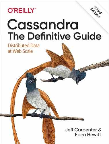
Now let’s say you want to spread replicas across multiple centers in case one of the data centers suffers some kind of catastrophic failure or network outage. The NetworkTopologyStrategy allows you to request that some replicas be placed in DC1, and some in DC2. Within each data center, the NetworkTopologyStrategy distributes replicas on distinct racks, because nodes in the same rack (or similar physical grouping) often fail at the same time due to power, cooling, or network issues.

The NetworkTopologyStrategy distributes the replicas as follows: the first replica is replaced according to the selected partitioner. Subsequent replicas are placed by traversing the nodes in the ring, skipping nodes in the same rack until a node in another rack is found. The process repeats for additional replicas, placing them on separate racks. Once a replica has been placed in each rack, the skipped nodes are used to place replicas until the replication factor has been met.

The NetworkTopologyStrategy allows you to specify a replication factor for each data center. Thus, the total number of replicas that will be stored is equal to the sum of the replication factors for each data center. The results of the NetworkTopologyStrategy are depicted in Figure 10-2.

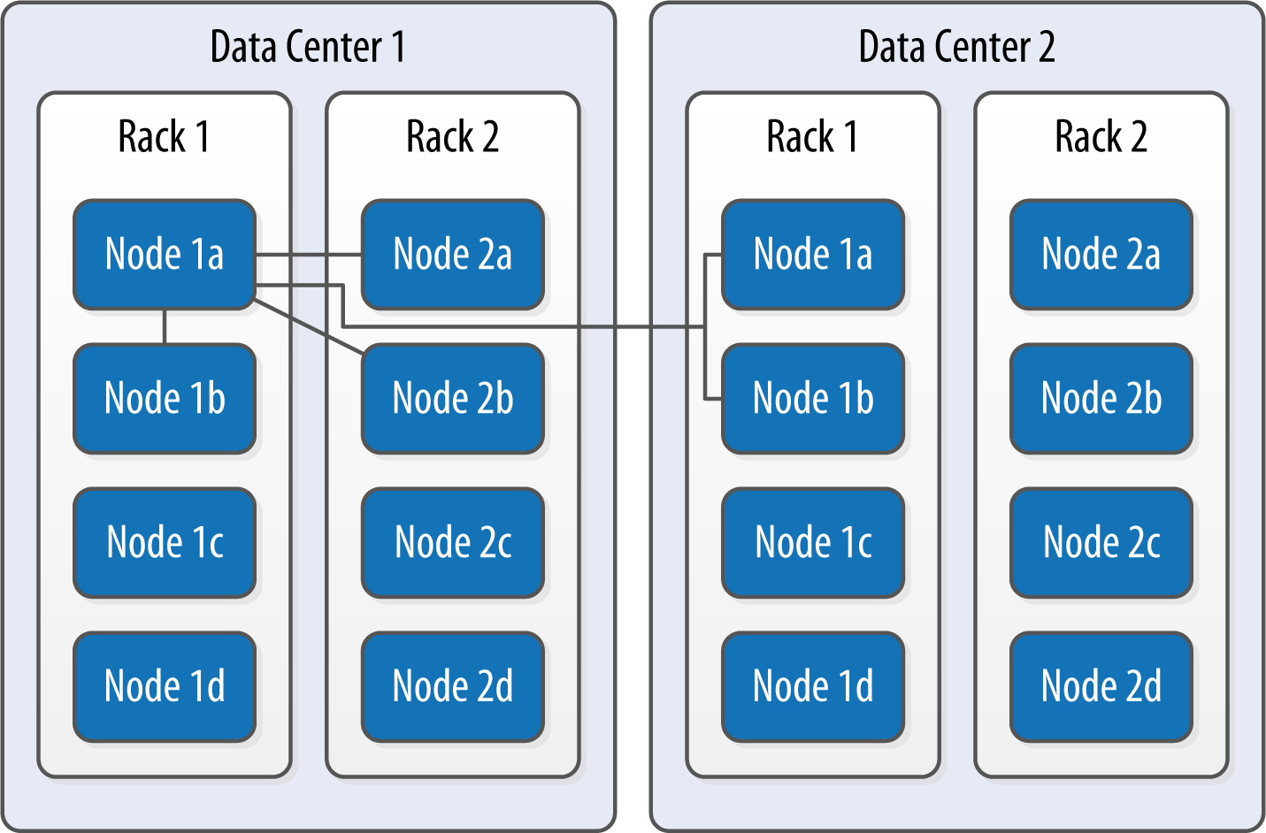
Figure 10-2. The NetworkTopologyStrategy places replicas in multiple data centers according to the specified replication factor per data center

To take advantage of additional data centers, you’ll need to update the replication strategy for the keyspaces in your cluster accordingly. For example, you might issue an ALTER KEYSPACE command to change the replication strategy for the reservation keyspace used by the Reservation Service:

cqlsh> ALTER KEYSPACE reservation
    WITH REPLICATION = {'class' : 'NetworkTopologyStrategy', 'DC1' : '3', 'DC2' : '3'};

Sizing Your Cluster

Next, consider the amount of data that your cluster will need to store. You will, of course, be able to add and remove nodes from your cluster in order to adjust its capacity over time, but calculating the initial and planned size over time will help you better anticipate costs and make sound decisions as you plan your cluster configuration.

In order to calculate the required size of the cluster, you’ll first need to determine the storage size of each of the supported tables using the formulas introduced in Chapter 5. This calculation is based on the columns within each table as well as the estimated number of rows and results in an estimated size of one copy of your data on disk.

In order to estimate the actual physical amount of disk storage required for a given table across your cluster, you’ll also need to consider the replication factor for the table’s keyspace and the compaction strategy in use. The resulting formula for the total size T_t is as follows:

$T_t=S_t*R{F}_k*CS{F}_t$

Where S_t is the size of the table calculated using the formula referenced above, RF_k is the replication factor of the keyspace, and CSF_t is a factor representing the compaction strategy of the table, whose value is as follows:

• 2 for the SizeTieredCompactionStrategy. The worst case scenario for this strategy is that there is a second copy of all of the data required for a major compaction.

• 1.25 for other compaction strategies, which have been estimated to require an extra 20% overhead during a major compaction.

Once you know the total physical disk size of the data for all tables, you can sum those values across all keyspaces and tables to arrive at the total data size for the cluster.

You can then divide this total by the amount of usable storage space per disk to estimate a required number of disks. A reasonable estimate for the usable storage space of a disk is 90% of the disk size. Historically, Cassandra operators have recommended 1TB as a maximum data size per node. This tends to provide a good balance between compute costs and time to complete operations such as compaction or streaming data to a new or replaced node. This may change in future releases.

Note that this calculation is based on the assumption of providing enough overhead on each disk to handle a major compaction of all keyspaces and tables. It’s possible to reduce the required overhead if you can ensure such a major compaction will never be executed by an operations team, but this seems like a risky assumption.

Once you’ve calculated the required size and number of nodes, you’ll be in a better position to decide on an initial cluster size. The amount of capacity you build into your cluster is dependent on how quickly you anticipate growth, which must be balanced against cost of additional hardware, whether it be physical or virtual.

Selecting Instances

It is important to choose the right computing resources for your Cassandra nodes, whether you’re running on physical hardware or in a virtualized cloud environment. The recommended computing resources for modern Cassandra releases (2.0 and later) tend to differ for development versus production environments:

Development environments

Cassandra nodes in development environments should generally have CPUs with at least two cores and 8 GB of memory. Although Cassandra has been successfully run on smaller processors such as Raspberry Pi with 512 MB of memory, this does require a significant performance-tuning effort.

Production environments

Cassandra nodes in production environments should have CPUs with at least eight cores and at least 32 GB of memory. Having additional cores tends to increase the throughput of both reads and writes.

Storage

There are a few factors to consider when selecting and configuring storage, including the type and quantities of drives to use:

HDDs versus SSDs

Cassandra supports both hard disk drives (HDDs, also called spinning drives) and solid state drives (SSDs) for storage. Although Cassandra’s usage of append-based writes is conducive to sequential writes on spinning drives, SSDs provide higher performance overall because of their support for low-latency random reads.

Historically, HDDs have been the more cost-effective storage option, but the cost of using SSDs has continued to come down, especially as more and more cloud platform providers support this as a storage option. Configure the disk_optimization_strategy in the cassandra.yaml file to either ssd (the default) or spinning as appropriate for your deployment.

Disk configuration

If you’re using spinning disks, it’s best to use separate disks for data and commit log files. If you’re using SSDs, the data and commit log files can be stored on the same disk.

JBOD vs RAID

Using servers with multiple disks is a recommended deployment pattern, with Just a Bunch of Disks (JBOD) or Redundant Array of Independent Disks (RAID) configurations. Because Cassandra uses replication to achieve redundancy across multiple nodes, the RAID 0 (or striped volume) configuration is considered sufficient. The JBOD approach provides the best overall performance and is a good choice if you have the ability to replace individual disks.

Use caution when considering shared storage

The standard recommendation for Cassandra deployments has been to avoid using Storage Area Networks (SAN) and Network Attached Storage (NAS). These storage technologies don’t scale as effectively as local storage—they consume additional network bandwidth in order to access the physical storage over the network, and they require additional I/O wait time on both reads and writes. However, we’ll consider possible exceptions to this rule below in “Cloud Deployment”.

Network

Because Cassandra relies on a distributed architecture involving multiple networked nodes, here are a few things you’ll need to consider:

Throughput

First, make sure your network is sufficiently robust to handle the traffic associated with distributing data across multiple nodes. The recommended network bandwidth is 1 GB or higher.

Network configuration

Make sure that you’ve correctly configured firewall rules and IP addresses for your nodes and network appliances to allow traffic on the ports used for the CQL native transport, inter-node communication (the listen_address), JMX, and so on. This includes networking between data centers (we’ll discuss cluster topology momentarily).

The clocks on all nodes should be synchronized using Network Time Protocol (NTP) or other methods. Remember that Cassandra only overwrites columns if the timestamp for the new value is more recent than the timestamp of the existing value. Without synchronized clocks, writes from nodes that lag behind can be lost.

Avoid load balancers

Load balancers are a feature of many computing environments. While these are frequently useful to spread incoming traffic across multiple service or application instances, it’s not recommended to use load balancers with Cassandra. Cassandra already provides its own mechanisms to balance network traffic between nodes, and the DataStax drivers spread client queries across replicas, so strictly speaking a load balancer won’t offer any additional help. Besides this, putting a load balancer in front of your Cassandra nodes actually introduces a potential single point of failure, which could reduce the availability of your cluster.

Timeouts

If you’re building a cluster that spans multiple data centers, it’s a good idea to measure the latency between data centers and tune timeout values in the cassandra.yaml file accordingly.

A proper network configuration is key to a successful Cassandra deployment, whether it is in a private data center, a public cloud spanning multiple data centers, or even a hybrid cloud environment.

Amazon Web Services

Amazon Web Services (AWS) has long been a popular deployment option for Cassandra, as evidenced by the presence of AWS-specific extensions in the Cassandra project such as the Ec2Snitch, Ec2MultiRegionSnitch, and the EC2MultiRegionAddressTranslator in the DataStax Java Driver.

Cluster layout

AWS is organized around the concepts of regions and availability zones, which are typically mapped to the Cassandra constructs of data centers and racks, respectively. A sample AWS cluster topology spanning the us-east-1 (Virginia) and eu-west-1 (Ireland) regions is shown in Figure 10-3. The node names are notional—this naming is not a required convention.

Figure 10-3. Topology of a cluster in two AWS regions

EC2 instances

The Amazon Elastic Compute Cloud (EC2) provides a variety of different virtual hardware instances grouped according to various classes. The two classes most frequently recommended for production Cassandra deployments are the C-class and the I-class, while the more general-purpose T-class and M-class instances are suitable for development and smaller production clusters.

The I-class instances are SSD-backed and designed for high I/O. These instances are ideal when using ephemeral storage, while the C-class instances are compute-optimized and suitable when using block storage. We’ll discuss these storage options below.

You can find more information about the various instance types available at https://docs.aws.amazon.com/AWSEC2/latest/UserGuide/instance-types.html.

Bitnami provides prebuilt Amazon Machine Images (AMIs) to simplify deployment, which you can find on their website or in the AWS Martketplace.

Data storage

The two options for storage in AWS EC2 are ephemeral storage attached to virtual instances and Elastic Block Store (EBS). The right choice for your deployment depend on factors including cost and operations.

The lower cost option is to use ephemeral storage. The drawback of this is that if an instance on which a node is running is terminated (as happens occasionally in AWS), the data is lost.

Alternatively, EBS volumes are a reliable place to store data that doesn’t go away when EC2 instances are dropped, and you can enable encryption on your volumes. However, reads will have some additional latency and your costs will be higher than ephemeral storage.

AWS Services such as S3 and Glacier are a good option for short- to medium-term and long-term storage of backups, respectively. On the other hand, it is quite simple to configure automatic backups of EBS volumes, which simplifies backup and recovery. You can create a new EBS volume from an existing snapshot.

Networking

If you’re running a multi-region configuration, you’ll want to make sure you have adequate networking between the regions. Many have found that using elements of the AWS Virtual Private Cloud (VPC) provides an effective way of achieving reliable, high-throughput connections between regions. AWS Direct Connect provides dedicated private networks, and there are virtual private network (VPN) options available as well. These services of course come at an additional cost.

If you have a single region deployment or a multi-region deployment using VPC peering, use the Ec2Snitch. If you have a multi-region deployment that uses public IP between regions, use the Ec2MultiRegionSnitch. Both EC2 snitches use the cassandra-rackdc.properties file, with data centers named after AWS regions (i.e. us-east-1) and racks named after availability zones (i.e. us-east-1a). For either snitch, increasing the phi_convict_threshold value in the cassandra.yaml file to 12 is generally recommended in the AWS network environment.

Additional guidance for deploying Cassandra on AWS can be found on the AWS Website.

Google Cloud Platform

Google Cloud Platform (GCP) provides cloud computing, application hosting, networking, storage, and various Software-as-a-Service (SaaS) offerings. In particular, GCP is well-known for its Big Data and Machine Learning services. You may wish to deploy (or extend) a Cassandra cluster into GCP in order to bring your data closer to these services.

Cluster layout

The Google Compute Environment (GCE) provides regions and zones, corresponding to Cassandra’s data centers and racks, respectively. Similar conventions for cluster layout apply as in AWS. Google Cloud StackDriver also provides a nice Cassandra integration for collecting and analyzing metrics.

Virtual machine instances

You can launch Cassandra quickly on the Google Cloud Platform using the Cloud Launcher. For example if you search the launcher at https://console.cloud.google.com/marketplace/browse?q=cassandra, you’ll find options for creating a cluster in just a few button clicks based on available VM images, and there are also options available to have a .

If you’re going to build your own images, GCE’s n1-standard and n1-highmem machine types are recommended for Cassandra deployments.

Data storage

GCE provides a variety of storage options for instances ranging from local spinning disk and SSD options for both ephemeral drives and network-attached drives.

Networking

You can deploy your cluster in a single global VPC network which can span regions on Google’s private network. You can also create connections between your own data centers and a Google VPC using Dedicated Interconnect or Partner Interconnect.

The GoogleCloudSnitch is a custom snitch designed just for the GCE, which also uses the cassandra-rackdc.properties file. The snitch may be used in a single region or across multiple regions. VPN networking is available between regions.

Microsoft Azure

Microsoft Azure is known as a cloud which is particularly well suited for enterprises, partly due to the large number of supported regions. Similar to GCP, there are a number of quick deployment options available in the Azure Marketplace.

Cluster layout

Azure provides data centers in locations worldwide, using the same term region as AWS. The concept of availability sets is used to manage collections of VMs. Azure manages the assignment of the VMs in an availability set across update domains, which equate to Cassandra’s racks.

Virtual machine instances

The Azure Resource Manager is recommended if you’re managing your own cluster deployments, since it enables specifying required resources declaratively.

Similar to AWS, Azure provides several classes of VMs. The D series VMs provide general purpose SSD-backed instances appropriate for most Cassandra deployments. The H series VMs provide additional memory as might be required for integrations such as the Apache Spark integration described in Chapter 15. You can find more information about Azure VM types at https://azure.microsoft.com/en-us/pricing/details/virtual-machines/linux/.

Data storage

Azure provides SSD, Premium SSD and HDD options on the previously mentioned instances. Premium SSDs are recommended for Cassandra nodes.

Networking

There is not a dedicated snitch for Azure. Instead, use the GossipingPropertyFileSnitch to allow your nodes to detect the cluster topology. For networking you may use public IPs, VPN Gateways or VNET Peering. VNET Peering is recommended as the best option, with peering of VNETs within a region or global peering across regions available.