
3
Maximizing and Minimizing
Goldilocks preferred the middle, but in the world of algorithms we’re usually more interested in the extreme highs and lows. Some powerful algorithms enable us to reach maxima (for example, maximum revenue, maximum profits, maximum efficiency, maximum productivity) and minima (for example, minimum cost, minimum error, minimum discomfort, and minimum loss). This chapter covers gradient ascent and gradient descent, two simple but effective methods to efficiently find maxima and minima of functions. We also discuss some of the issues that come with maximization and minimization problems, and how to deal with them. Finally, we discuss how to know whether a particular algorithm is appropriate to use in a given situation. We’ll start with a hypothetical scenario—trying to set optimal tax rates to maximize a government’s revenues—and we’ll see how to use an algorithm to find the right solution.
Setting Tax Rates
Imagine that you’re elected prime minister of a small country. You have ambitious goals, but you don’t feel like you have the budget to achieve them. So your first order of business after taking office is to maximize the tax revenues your government brings in.
It’s not obvious what taxation rate you should choose to maximize revenues. If your tax rate is 0 percent, you will get zero revenue. At 100 percent, it seems likely that taxpayers would avoid productive activity and assiduously seek tax shelters to the point that revenue would be quite close to zero. Optimizing your revenue will require finding the right balance between rates that are so high that they discourage productive activity and rates that are so low that they undercollect. To achieve that balance is, you’ll need to know more about the way tax rates relate to revenue.
Steps in the Right Direction
Suppose that you discuss this with your team of economists. They see your point and retire to their research office, where they consult the apparatuses used by top-level research economists everywhere—mostly test tubes, hamsters running on wheels, astrolabes, and dowsing rods—to determine the precise relationship between tax rates and revenues.
After some time thus sequestered, the team tells you that they’ve determined a function that relates the taxation rate to the revenue collected, and they’ve been kind enough to write it in Python for you. Maybe the function looks like the following:
import math
def revenue(tax):
    return(100 * (math.log(tax+1) - (tax - 0.2)**2 + 0.04))
This is a Python function that takes tax as its argument and returns a numeric output. The function itself is stored in a variable called revenue. You fire up Python to generate a simple graph of this curve, entering the following in the console. Just as in Chapter 1, we’ll use the matplotlib module for its plotting capabilities.
import matplotlib.pyplot as plt
xs = [x/1000 for x in range(1001)]
ys = [revenue(x) for x in xs]
plt.plot(xs,ys)
plt.title('Tax Rates and Revenue')
plt.xlabel('Tax Rate')
plt.ylabel('Revenue')
plt.show()
This plot shows the revenues (in billions of your country’s currency) that your team of economists expects for each tax rate between 0 and 1 (where 1 represents a 100 percent tax rate). If your country currently has a flat 70 percent tax on all income, we can add two lines to our code to plot that point on the curve as follows:
import matplotlib.pyplot as plt
xs = [x/1000 for x in range(1001)]
ys = [revenue(x) for x in xs]
plt.plot(xs,ys)
current_rate = 0.7
plt.plot(current_rate,revenue(current_rate),'ro')
plt.title('Tax Rates and Revenue')
plt.xlabel('Tax Rate')
plt.ylabel('Revenue')
plt.show()
The final output is the simple plot in Figure 3-1.
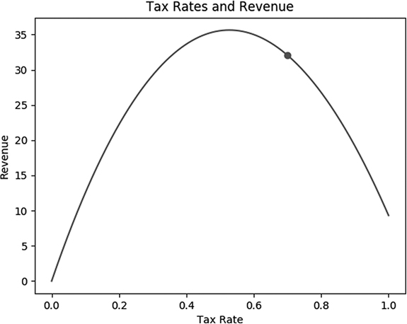
Figure 3-1: The relationship between tax rates and revenue, with a dot representing your country’s current situation
Your country’s current tax rate, according to the economists’ formula, is not quite maximizing the government’s revenue. Although a simple visual inspection of the plot will indicate approximately what level corresponds to the maximum revenue, you are not satisfied with loose approximations and you want to find a more precise figure for the optimal tax rate. It’s apparent from the plot of the curve that any increase from the current 70 percent rate should decrease total revenues, and some amount of decrease from the current 70 percent rate should increase total revenues, so in this situation, revenue maximization will require a decrease in the overall tax rate.
We can verify whether this is true more formally by taking the derivative of the economists’ revenue formula. A derivative is a measurement of the slope of a tangent line, with large values denoting steepness and negative values denoting downward motion. You can see an illustration of a derivative in Figure 3-2: it’s just a way to measure how quickly a function is growing or shrinking.
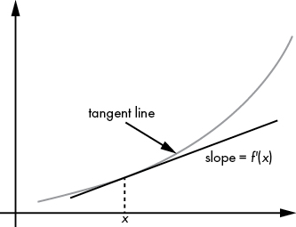
Figure 3-2: To calculate a derivative, we take a tangent line to a curve at a point and find its slope.
We can create a function in Python that specifies this derivative as follows:
def revenue_derivative(tax):
    return(100 * (1/(tax + 1) - 2 * (tax - 0.2)))
We used four rules of calculus to derive that function. First, we used the rule that the derivative of log(x) is 1/x. That’s why the derivative of log(tax + 1) is 1/(tax + 1). Another rule is that the derivative of x2 is 2x. That’s why the derivative of (tax – 0.2)2 is 2(tax – 0.2). Two more rules are that the derivative of a constant number is always 0, and the derivative of 100f(x) is 100 times the derivative of f(x). If you combine all these rules, you’ll find that our tax-revenue function, 100(log(tax + 1) – (tax – 0.2)2 + 0.04), has a derivative equal to the following, as described in the Python function:

We can check that the derivative is indeed negative at the country’s current taxation rate:
print(revenue_derivative(0.7))This gives us the output -41.17647.
A negative derivative means that an increase in tax rate leads to a decrease in revenue. By the same token, a decrease in tax rate should lead to an increase in revenue. While we are not yet sure of the precise tax rate corresponding to the maximum of the curve, we can at least be sure that if we take a small step from where are in the direction of decreased taxation, revenue should increase.
To take a step toward the revenue maximum, we should first specify a step size. We can store a prudently small step size in a variable in Python as follows:
step_size = 0.001Next, we can take a step in the direction of the maximum by finding a new rate that is proportional to one step size away from our current rate, in the direction of the maximum:
current_rate = current_rate + step_size * revenue_derivative(current_rate)Our process so far is that we start at our current tax rate and take a step toward the maximum whose size is proportional to the step_size we chose and whose direction is determined by the derivative of the tax-revenue function at the current rate.
We can verify that after this step, the new current_rate is 0.6588235 (about a 66 percent tax rate), and the revenue corresponding to this new rate is 33.55896. But while we have taken a step toward the maximum and increased the revenue, but we find ourselves in essentially the same situation as before: we are not yet at the maximum, but we know the derivative of the function and the general direction in which we should travel to get there. So we simply need to take another step, exactly as before but with the values representing the new rate. Yet again we set:
current_rate = current_rate + step_size * revenue_derivative(current_rate)After running this again, we find that the new current_rate is 0.6273425, and the revenue corresponding to this new rate is 34.43267. We have taken another step in the right direction. But we are still not at the maximum revenue rate, and we will have to take another step to get closer.
Turning the Steps into an Algorithm
You can see the pattern that is emerging. We’re following these steps repeatedly:
- Start with a
current_rateand astep_size. - Calculate the derivative of the function you are trying to maximize at the
current_rate. - Add
step_size*revenue_derivative(current_rate) to the current rate, to get a newcurrent_rate. - Repeat steps 2 and 3.
The only thing that’s missing is a rule for when to stop, a rule that triggers when we have reached the maximum. In practice, it’s quite likely that we’ll be asymptotically approaching the maximum: getting closer and closer to it but always remaining microscopically distant. So although we may never reach the maximum, we can get close enough that we match it up to 3 or 4 or 20 decimal places. We will know when we are sufficiently close to the asymptote when the amount by which we change our rate is very small. We can specify a threshold for this in Python:
threshold = 0.0001Our plan is to stop our process when we are changing the rate by less than this amount at each iteration of our process. It’s possible that our step-taking process will never converge to the maximum we are seeking, so if we set up a loop, we’ll get stuck in an infinite loop. To prepare for this possibility, we’ll specify a number of “maximum iterations,” and if we take a number of steps equal to this maximum, we’ll simply give up and stop.
Now, we can put all these steps together (Listing 3-1).
threshold = 0.0001
maximum_iterations = 100000

keep_going = True
iterations = 0
while(keep_going):
    rate_change = step_size * revenue_derivative(current_rate)
    current_rate = current_rate + rate_change

    if(abs(rate_change) < threshold):
        keep_going = False

    if(iterations >= maximum_iterations):
        keep_going = False

    iterations = iterations+1
Listing 3-1: Implementing gradient ascent
After running this code, you’ll find that the revenue-maximizing tax rate is about 0.528. What we’ve done in Listing 3-1 is something called gradient ascent. It’s called that because it’s used to ascend to a maximum, and it determines the direction of movement by taking the gradient. (In a two-dimensional case like ours, a gradient is simply called a derivative.) We can write out a full list of the steps we followed here, including a description of our stopping criteria:
- Start with a
current_rateand astep_size. - Calculate the derivative of the function you are trying to maximize at the
current_rate. - Add
step_size * revenue_derivative(current_rate) to the current rate, to get a newcurrent_rate. - Repeat steps 2 and 3 until you are so close to the maximum that your current tax rate is changing less than a very small threshold at each step, or until you have reached a number of iterations that is sufficiently high.
Our process can be written out simply, with only four steps. Though humble in appearance and simple in concept, gradient ascent is an algorithm, just like the algorithms described in previous chapters. Unlike most of those algorithms, though, gradient ascent is in common use today and is a key part of many of the advanced machine learning methods that professionals use daily.
Objections to Gradient Ascent
We’ve just performed gradient ascent to maximize the revenues of a hypothetical government. Many people who learn gradient ascent have practical if not moral objections to it. Here are some of the arguments that people raise about gradient ascent:
- It’s unnecessary because we can do a visual inspection to find the maximum.
- It’s unnecessary because we can do repeated guesses, a guess-and-check strategy, to find the maximum.
- It’s unnecessary because we can solve the first-order conditions.
Let’s consider each of these objections in turn. We discussed visual inspection previously. For our taxation/revenue curve, it’s easy to get an approximate idea of the location of a maximum through visual inspection. But visual inspection of a plot does not enable high precision. More importantly, our curve is extremely simple: it can be plotted in two dimensions and obviously has only one maximum on the range that interests us. If you imagine more complex functions, you can start to see why visual inspection is not a satisfactory way to find the maximum value of a function.
For example, consider a multidimensional case. If our economists had concluded that revenue depended not only on tax rates but also on tariff rates, then our curve would have to be drawn in three dimensions, and if it were a complex function, it could be harder to see where the maximum lies. If our economists had created a function that related 10 or 20 or a 100 predictors to expected revenue, it would not be possible to draw a plot of all of them simultaneously given the limitations of our universe, our eyes, and our brains. If we couldn’t even draw the tax/revenue curve, then there’s no way visual inspection could enable us to find its maximum. Visual inspection works for simple toy examples like the tax/revenue curve, but not for highly complex multidimensional problems. Besides all of that, plotting a curve itself requires calculating the function’s value at every single point of interest, so it always takes longer than a well-written algorithm.
It may seem that gradient ascent is overcomplicating the issue, and that a guess-and-check strategy is sufficient for finding the maximum. A guess-and-check strategy would consist of guessing a potential maximum and checking whether it is higher than all previously guessed candidate maxima until we are confident that we have found the maximum. One potential reply to this is to point out that, just as with visual inspections, with high-complexity multidimensional functions, guess-and-check could be prohibitively difficult to successfully implement in practice. But the best reply to the idea of guessing and checking to find maxima is that this is exactly what gradient ascent is already doing. Gradient ascent already is a guess-and-check strategy, but one that is “guided” by moving guesses in the direction of the gradient rather than by guessing randomly. Gradient ascent is just a more efficient version of guess-and-check.
Finally, consider the idea of solving the first-order conditions to find a maximum. This is a method that is taught in calculus classes all around the world. It could be called an algorithm, and its steps are:
- Find the derivative of the function you are trying to maximize.
- Set that derivative equal to zero.
- Solve for the point at which the derivative is equal to zero.
- Make sure that point is a maximum rather than a minimum.
(In multiple dimensions, we can work with a gradient instead of a derivative and perform an analogous process.) This optimization algorithm is fine as far as it goes, but it could be difficult or impossible to find a closed-form solution for which a derivative is equal to zero (step 2), and it could be harder to find that solution than it would be to simply perform gradient ascent. Besides that, it could take huge computing resources, including space, processing power, or time, and not all software has symbolic algebra capabilities. In that sense, gradient ascent is more robust than this algorithm.
The Problem of Local Extrema
Every algorithm that tries to find a maximum or minimum faces a very serious potential problem with local extrema (local maximums and minimums). We may perform gradient ascent perfectly, but realize that the peak we have reached at the end is only a “local” peak—it’s higher than every point around it, but not higher than some faraway global maximum. This could happen in real life as well: you try to climb a mountain, you reach a summit where you are higher than all of your immediate surroundings, but you realize that you’re only on the foothill and the real summit is far away and much higher. Paradoxically, you may have to walk down a little to eventually get to that higher summit, so the “naive” strategy that gradient ascent follows, always stepping to a slightly higher point in one’s immediate neighborhood, fails to get to the global maximum.
Education and Lifetime Income
Local extrema are a very serious problem in gradient ascent. As an example, consider trying to maximize lifelong income by choosing the optimal level of education. In this case, we might suppose that lifelong earnings relate to years of education according to the following formula:
import math
def income(edu_yrs):
    return(math.sin((edu_yrs - 10.6) * (2 * math.pi/4)) + (edu_yrs - 11)/2)
Here, edu_yrs is a variable expressing how many years of education one has received, and income is a measurement of one’s lifetime income. We can plot this curve as follows, including a point for a person who has 12.5 years of formal education—that is, someone who has graduated from high school (12 years of formal education) and is half a year into a bachelor’s degree program:
import matplotlib.pyplot as plt
xs = [11 + x/100 for x in list(range(901))]
ys = [income(x) for x in xs]
plt.plot(xs,ys)
current_edu = 12.5
plt.plot(current_edu,income(current_edu),'ro')
plt.title('Education and Income')
plt.xlabel('Years of Education')
plt.ylabel('Lifetime Income')
plt.show()
We get the graph in Figure 3-3.
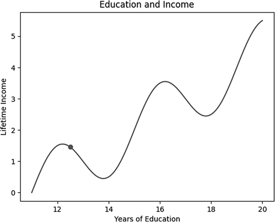
Figure 3-3: The relationship between formal education and lifetime income
This graph, and the income function used to generate it, is not based on empirical research but is used only as an illustrative, purely hypothetical example. It shows what might be intuitive relationships between education and income. Lifetime income is likely to be low for someone who does not graduate from high school (has fewer than 12 years of formal education). Graduation from high school—12 years—is an important milestone and should correspond to higher earnings than dropping out. In other words, it’s a maximum, but importantly it’s only a local maximum. Getting more than 12 years of education is helpful, but not at first. Someone who has completed only a few months of college education is not likely to get jobs that differ from those available to a high school graduate, but by going to school for extra months, they’ve missed an opportunity to earn in those months, so their lifetime earnings are actually lower than the earnings of people who enter the workforce directly after high school graduation and remain there.
Only after several years of college education does someone acquire skills that enable them to earn more over a lifetime than a high school graduate after we take into account the lost earning potential of the years spent at school. Then, college graduates (at 16 years of education) are at another earnings peak higher than the local high school peak. Once again, it’s only a local one. Getting a little more education after earning a bachelor’s degree leads to the same situation as getting a little more education after a high school diploma: you don’t immediately acquire enough skills to compensate for the time not spent earning. Eventually, that’s reversed, and you reach what looks like another peak after obtaining a postgraduate degree. It’s hard to speculate much further beyond that, but this simplistic view of education and earnings will suffice for our purposes.
Climbing the Education Hill—the Right Way
For the individual we’ve imagined, drawn at 12.5 years of education on our graph, we can perform gradient ascent exactly as outlined previously. Listing 3-2 has a slightly altered version of the gradient ascent code we introduced in Listing 3-1.
def income_derivative(edu_yrs):
    return(math.cos((edu_yrs - 10.6) * (2 * math.pi/4)) + 1/2)

threshold = 0.0001
maximum_iterations = 100000

current_education = 12.5
step_size = 0.001

keep_going = True
iterations = 0
while(keep_going):
    education_change = step_size * income_derivative(current_education)
    current_education = current_education + education_change
    if(abs(education_change) < threshold):
        keep_going = False
    if(iterations >= maximum_iterations):
        keep_going=False
    iterations = iterations + 1
Listing 3-2: An implementation of gradient ascent that climbs an income hill instead of a revenue hill
The code in Listing 3-2 follows exactly the same gradient ascent algorithm as the revenue-maximization process we implemented previously. The only difference is the curve we are working with. Our taxation/revenue curve had one global maximum value that was also the only local maximum. Our education/income curve, by contrast, is more complicated: it has a global maximum, but also several local maximum values (local peaks or maxima) that are lower than the global maximum. We have to specify the derivative of this education/income curve (in the first lines of Listing 3-2), we have a different initial value (12.5 years of education instead of 70 percent taxation), and we have different names for the variables (current_education instead of current_rate). But these differences are superficial; fundamentally we are doing the same thing: taking small steps in the direction of the gradient toward a maximum until we reach an appropriate stopping point.
The outcome of this gradient ascent process is that we conclude that this person is overeducated, and actually about 12 years is the income-maximizing number of years of education. If we are naive and trust the gradient ascent algorithm too much, we might recommend that college freshmen drop out and join the workforce immediately to maximize earnings at this local maximum. This is a conclusion that some college students have come to in the past, as they see their high school–graduate friends making more money than them as they work toward an uncertain future. Obviously, this is not right: our gradient ascent process has found the top of a local hill, but not the global maximum. The gradient ascent process is depressingly local: it climbs only the hill it’s on, and it isn’t capable of taking temporary steps downward for the sake of eventually getting to another hill with a higher peak. There are some analogues to this in real life, as with people who fail to complete a university degree because it will prevent them from earning in the near term. They don’t consider that their long-term earnings will be improved if they push through a local minimum to another hill to climb (their next, more valuable degree).
The local extrema problem is a serious one, and there’s no silver bullet for resolving it. One way to attack the problem is to attempt multiple initial guesses and perform gradient ascent for each of them. For example, if we performed gradient ascent for 12.5, 15.5, and 18.5 years of education, we would get different results each time, and we could compare these results to see that in fact the global maximum comes from maximizing years of education (at least on this scale).
This is a reasonable way to deal with the local extremum problem, but it can take too long to perform gradient ascent enough times to get the right maximum, and we’re never guaranteed to get the right answer even after hundreds of attempts. An apparently better way to avoid the problem is to introduce some degree of randomness into the process, so that we can sometimes step in a way that leads to a locally worse solution, but which in the long term can lead us to better maxima. An advanced version of gradient ascent, called stochastic gradient ascent, incorporates randomness for this reason, and other algorithms, like simulated annealing, do the same. We’ll discuss simulated annealing and the issues related to advanced optimization in Chapter 6. For now, just keep in mind that as powerful as gradient ascent is, it will always face difficulties with the local extrema problem.
From Maximization to Minimization
So far we’ve sought to maximize revenue: to climb a hill and to ascend. It’s reasonable to wonder whether we would ever want to go down a hill, to descend and to minimize something (like cost or error). You might think that a whole new set of techniques is required for minimization or that our existing techniques need to be flipped upside down, turned inside out, or run in reverse.
In fact, moving from maximization to minimization is quite simple. One way to do it is to “flip” our function or, more precisely, to take its negative. Going back to our tax/revenue curve example, it is as simple as defining a new flipped function like so:
def revenue_flipped(tax):
    return(0 - revenue(tax))
We can then plot the flipped curve as follows:
import matplotlib.pyplot as plt
xs = [x/1000 for x in range(1001)]
ys = [revenue_flipped(x) for x in xs]
plt.plot(xs,ys)
plt.title('The Tax/Revenue Curve - Flipped')
plt.xlabel('Current Tax Rate')
plt.ylabel('Revenue - Flipped')
plt.show()
Figure 3-4 shows the flipped curve.
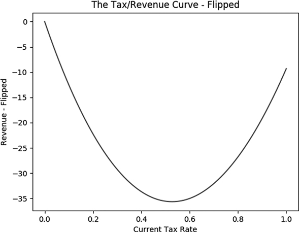
Figure 3-4: The negative or “flipped” version of the tax/revenue curve
So if we want to maximize the tax/revenue curve, one option is to minimize the flipped tax/revenue curve. If we want to minimize the flipped tax/revenue curve, one option is to maximize the flipped flipped curve—in other words, the original curve. Every minimization problem is a maximization problem of a flipped function, and every maximization problem is a minimization of a flipped function. If you can do one, you can do the other (after flipping). Instead of learning to minimize functions, you can just learn to maximize them, and every time you are asked to minimize, maximize the flipped function instead and you’ll get the right answer.
Flipping is not the only solution. The actual process of minimization is very similar to the process of maximization: we can use gradient descent instead of gradient ascent. The only difference is the direction of movement at each step; in gradient descent, we go down instead of up. Remember that to find the maximum of the tax/revenue curve, we move in the direction of the gradient. In order to minimize, we move in the opposite direction of the gradient. This means we can alter our original gradient ascent code as in Listing 3-3.
threshold = 0.0001
maximum_iterations = 10000

def revenue_derivative_flipped(tax):
    return(0-revenue_derivative(tax))

current_rate = 0.7

keep_going = True
iterations = 0
while(keep_going):
    rate_change = step_size * revenue_derivative_flipped(current_rate)
    current_rate = current_rate - rate_change
    if(abs(rate_change) < threshold):
        keep_going = False
    if(iterations >= maximum_iterations):
        keep_going = False
    iterations = iterations + 1
Listing 3-3: Implementating gradient descent
Here everything is the same except we have changed a + to a - when we change the current_rate. By making this very small change, we’ve converted gradient ascent code to gradient descent code. In a way, they’re essentially the same thing; they use a gradient to determine a direction, and then they move in that direction toward a definite goal. In fact, the most common convention today is to speak of gradient descent, and to refer to gradient ascent as a slightly altered version of gradient descent, the opposite of how this chapter has introduced it.
Hill Climbing in General
Being elected prime minister is a rare occurrence, and setting taxation rates to maximize government revenue is not an everyday activity even for prime ministers. (For the real-life version of the taxation/revenue discussion at the beginning of the chapter, I encourage you to look up the Laffer curve.) However, the idea of maximizing or minimizing something is extremely common. Businesses attempt to choose prices to maximize profits. Manufacturers attempt to choose practices that maximize efficiency and minimize defects. Engineers attempt to choose design features that maximize performance or minimize drag or cost. Economics is largely structured around maximization and minimization problems: maximizing utility especially, and also maximizing dollar amounts like GDP and revenue, and minimizing estimation error. Machine learning and statistics rely on minimization for the bulk of their methods; they minimize a “loss function” or an error metric. For each of these, there is the potential to use a hill-climbing solution like gradient ascent or descent to get to an optimal solution.
Even in everyday life, we choose how much money to spend to maximize achievement of our financial goals. We strive to maximize happiness and joy and peace and love and minimize pain and discomfort and sadness.
For a vivid and relatable example, think of being at a buffet and seeking, as all of us do, to eat the right amount to maximize satisfaction. If you eat too little, you will walk out hungry and you may feel that by paying the full buffet price for only a little food, you haven’t gotten your money’s worth. If you eat too much, you will feel uncomfortable and maybe even sick, and maybe you will violate your self-imposed diet. There is a sweet spot, like the peak of the tax/revenue curve, that is the exact amount of buffet consumption that maximizes satisfaction.
We humans can feel and interpret sensory input from our stomachs that tells us whether we’re hungry or full, and this is something like a physical equivalent of taking a gradient of a curve. If we’re too hungry, we take some step with a predecided size, like one bite, toward reaching the sweet spot of satisfaction. If we’re too full, we stop eating; we can’t “un-eat” something we have already eaten. If our step size is small enough, we can be confident that we will not overstep the sweet spot by much. The process we go through when we are deciding how much to eat at a buffet is an iterative process involving repeated direction checks and small steps in adjustable directions—in other words, it’s essentially the same as the gradient ascent algorithm we studied in this chapter.
Just as with the example of catching balls, we see in this buffet example that algorithms like gradient ascent are natural to human life and decision-making. They are natural to us even if we have never taken a math class or written a line of code. The tools in this chapter are merely meant to formalize and make precise the intuitions you already have.
When Not to Use an Algorithm
Often, learning an algorithm fills us with a feeling of power. We feel that if we are ever in a situation that requires maximization or minimization, we should immediately apply gradient ascent or descent and implicitly trust whatever results we find. However, sometimes more important than knowing an algorithm is knowing when not to use it, when it’s inappropriate or insufficient for the task at hand, or when there is something better that we should try instead.
When should we use gradient ascent (and descent), and when should we not? Gradient ascent works well if we start with the right ingredients:
- A mathematical function to maximize
- Knowledge of where we currently are
- An unequivocal goal to maximize the function
- Ability to alter where we are
There are many situations in which one or more of these ingredients is missing. In the case of setting taxation rates, we used a hypothetical function relating tax rates to revenue. However, there’s no consensus among economists about what that relationship is and what functional form it takes. So we can perform gradient ascent and descent all we like, but until we can all agree on what function we need to maximize, we cannot rely on the results we find.
In other situations, we may find that gradient ascent isn’t very useful because we don’t have the ability to take action to optimize our situation. For example, suppose that we derived an equation relating a person’s height to their happiness. Maybe this function expresses how people who are too tall suffer because they cannot get comfortable on airplanes, and people who are too short suffer because they cannot excel at pickup basketball games, but some sweet spot in the middle of too tall and too short tends to maximize happiness. Even if we can express this function perfectly and apply gradient ascent to find the maximum, it will not be useful to us, because we do not have control over our height.
If we zoom out even further, we may have all the ingredients required for gradient ascent (or any other algorithm) and still wish to refrain for deeper philosophical reasons. For example, suppose you can precisely determine a tax-revenue function and you’re elected prime minister with full control over the taxation rate in your country. Before you apply gradient ascent and climb to the revenue-maximizing peak, you may want to ask yourself if maximizing your tax revenue is the right goal to pursue in the first place. It could be that you are more concerned with freedom or economic dynamism or redistributive justice or even opinion polls than you are with state revenues. Even if you have decided that you want to maximize revenues, it’s not clear that maximizing revenues in the short term (that is, this year) will lead to maximization of revenues in the long term.
Algorithms are powerful for practical purposes, enabling us to achieve goals like catching baseballs and finding revenue-maximizing taxation rates. But though algorithms can achieve goals effectively, they’re not as suited to the more philosophical task of deciding which goals are worth pursuing in the first place. Algorithms can make us clever, but they cannot make us wise. It’s important to remember that the great power of algorithms is useless or even harmful if it is used for the wrong ends.
Summary
This chapter introduced gradient ascent and gradient descent as simple and powerful algorithms used to find the maxima and minima of functions, respectively. We also talked about the serious potential problem of local extrema, and some philosophical considerations about when to use algorithms and when to gracefully refrain.
Hang on tight, because in the next chapter we discuss a variety of searching and sorting algorithms. Searching and sorting are fundamental and important in the world of algorithms. We’ll also talk about “big O” notation and the standard ways to evaluate algorithm performance.