
10
Artificial Intelligence
Throughout this book, we’ve noted the capacity of the human mind to do remarkable things, whether it be catching baseballs, proofreading texts, or deciding whether someone is having a heart attack. We explored the ways we can translate these abilities into algorithms, and the challenges therein. In this chapter, we face these challenges once more and build an algorithm for artificial intelligence (AI). The AI algorithm we’ll discuss will be applicable not only to one narrow task, like catching a baseball, but to a wide range of competitive scenarios. This broad applicability is what excites people about artificial intelligence—just as a human can learn new skills throughout life, the best AI can apply itself to domains it’s never seen before with only minimal reconfiguration.
The term artificial intelligence has an aura about it that can make people think that it’s mysterious and highly advanced. Some believe that AI enables computers to think, feel, and experience conscious thought in the same way that humans do; whether computers will ever be able to do so is an open, difficult question that is far beyond the scope of this chapter. The AI that we’ll build is much simpler and will be capable of playing a game well, but not of writing sincerely felt love poems or feeling despondency or desire (as far as I can tell!).
Our AI will be able to play dots and boxes, a simple but nontrivial game played worldwide. We’ll start by drawing the game board. Then we’ll build functions to keep score as games are in progress. Next, we’ll generate game trees that represent all possible combinations of moves that can be played in a given game. Finally, we’ll introduce the minimax algorithm, an elegant way to implement AI in just a few lines.
La Pipopipette
Dots and boxes was invented by the French mathematician Édouard Lucas, who named it la pipopipette. It starts with a lattice, or grid of points, like the one shown in Figure 10-1.
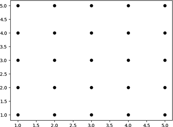
Figure 10-1: A lattice, which we can use as a game board for dots and boxes
The lattice is usually a rectangle but can be any shape. Two players play against each other, taking turns. On each turn, a player is allowed to draw a line segment that connects two adjacent points in the lattice. If they use different colors to draw their line segments, we can see who has drawn what, though that’s not required. As they proceed through the game, line segments fill the lattice until every possible segment connecting adjacent points is drawn. You can see an example game in progress in Figure 10-2.
A player’s goal in dots and boxes is to draw line segments that complete squares. In Figure 10-2, you can see that in the bottom left of the game board, one square has been completed. Whichever player drew the line segment that completed that square will have earned one point from doing so. In the top-right section, you can see that three sides of another square have been drawn. It’s player one’s turn, and if they use their turn to draw a line segment between (4,4) and (4,3), they’ll earn one point for that. If instead they draw another line segment, like a line segment from (4,1) to (5,1), then they’ll give they’ll give player two a chance to finish the square and earn a point. Players only earn points for completing the smallest possible squares on the board: those with a side length of 1. The player who’s earned the most points when the lattice is completely filled in with line segments wins the game. There are some variations on the game, including different board shapes and more advanced rules, but the simple AI we’ll build in this chapter will work with the rules we’ve described here.
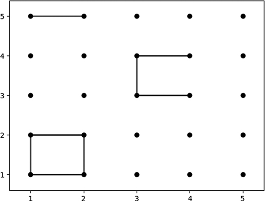
Figure 10-2: A dots and boxes game in progress
Drawing the Board
Though not strictly necessary for our algorithmic purposes, drawing the board can make it easier to visualize the ideas we’re discussing. A very simple plotting function can make an n×n lattice by looping over x and y coordinates and using the plot() function in Python’s matplotlib module:
import matplotlib.pyplot as plt
from matplotlib import collections as mc
def drawlattice(n,name):
    for i in range(1,n + 1):
        for j in range(1,n + 1):
            plt.plot(i,j,'o',c = 'black')
    plt.savefig(name)
In this code, n represents the size of each side of our lattice, and we use the name argument for the filepath where we want to save the output. The c = 'black' argument specifies the color of the points in our lattice. We can create a 5×5 black lattice and save it with the following command:
drawlattice(5,'lattice.png')This is exactly the command that was used to create Figure 10-1.
Representing Games
Since a game of dots and boxes consists of successively drawn line segments, we can record a game as a list of ordered lines. Just as we did in previous chapters, we can represent a line (one move) as a list consisting of two ordered pairs (the ends of the line segment). For example, we can represent the line between (1,2) and (1,1) as this list:
[(1,2),(1,1)]A game will be an ordered list of such lines, like the following example:
game = [[(1,2),(1,1)],[(3,3),(4,3)],[(1,5),(2,5)],[(1,2),(2,2)],[(2,2),(2,1)],[(1,1),(2,1)], [(3,4),(3,3)],[(3,4),(4,4)]]This game is the one illustrated in Figure 10-2. We can tell it must still be in progress, since not all of the possible line segments have been drawn to fill in the lattice.
We can add to our drawlattice() function to create a drawgame() function. This function should draw the points of the game board as well as all line segments that have been drawn between them in the game so far. The function in Listing 10-1 will do the trick.
def drawgame(n,name,game):
    colors2 = []
    for k in range(0,len(game)):
        if k%2 == 0:
            colors2.append('red')
        else:
            colors2.append('blue')
    lc = mc.LineCollection(game, colors = colors2, linewidths = 2)
    fig, ax = plt.subplots()
    for i in range(1,n + 1):
        for j in range(1,n + 1):
            plt.plot(i,j,'o',c = 'black')
    ax.add_collection(lc)
    ax.autoscale()
    ax.margins(0.1)
    plt.savefig(name)
Listing 10-1: A function that draws a game board for dots and boxes
This function takes n and name as arguments, just as drawlattice() did. It also includes exactly the same nested loops we used to draw lattice points in drawlattice(). The first addition you can see is the colors2 list, which starts out empty, and we fill it up with the colors we assign to the line segments that we’ll draw. In dots and boxes, turns alternate between the two players, so we’ll alternate the colors of the line segments that we assign to the players—in this case, red for the first player and blue for the second player. The for loop after the definition of the colors2 list fills it up with alternating instances of 'red' and 'blue' until there are as many color assignments as there are moves in the game. The other lines of code we’ve added create a collection of lines out of our game moves and draw them, in the same way we’ve drawn collections of lines in previous chapters.
We can call our drawgame() function in one line as follows:
drawgame(5,'gameinprogress.png',game)This is exactly how we created Figure 10-2.
Scoring Games
Next, we’ll create a function that can keep score for a dots and boxes game. We start with a function that can take any given game and find the completed squares that have been drawn, and then we create a function that will calculate the score. Our function will count completed squares by iterating over every line segment in the game. If a line is a horizontal line, we determine whether it is the top of a completely drawn square by checking whether the parallel line below it has also been drawn in the game, and also whether the left and right sides of the square have been drawn. The function in Listing 10-2 accomplishes this:
def squarefinder(game):
    countofsquares = 0
    for line in game:
        parallel = False
        left=False
        right=False
        if line[0][1]==line[1][1]:
            if [(line[0][0],line[0][1]-1),(line[1][0],line[1][1] - 1)] in game:
                parallel=True
            if [(line[0][0],line[0][1]),(line[1][0]-1,line[1][1] - 1)] in game:
                left=True
            if [(line[0][0]+1,line[0][1]),(line[1][0],line[1][1] - 1)] in game:
                right=True
            if parallel and left and right:
                countofsquares += 1
    return(countofsquares)
Listing 10-2: A function that counts the number of squares that appear in a dots and boxes game board
You can see that the function returns the value of countofsquares, which we initialized with a 0 value at the beginning of the function. The function’s for loop iterates over every line segment in a game. We start out assuming that neither the parallel line below this line nor the left and right lines that would connect these parallel lines have been played in the game so far. If a given line is a horizontal line, we check for the existence of those parallel, left, and right lines. If all four lines of the square we’ve checked are listed in the game, then we increment the countofsquares variable by 1. In this way, countofsquares records the total number of squares that have been completely drawn in the game so far.
Now we can write a short function to calculate the score of a game. The score will be recorded as a list with two elements, like [2,1]. The first element of the score list represents the score of the first player, and the second element represents the score of the second player. Listing 10-3 has our scoring function.
def score(game):
    score = [0,0]
    progress = []
    squares = 0
    for line in game:
        progress.append(line)
        newsquares = squarefinder(progress)
        if newsquares > squares:
            if len(progress)%2 == 0:
                score[1] = score[1] + 1
            else:
                score[0] = score[0] + 1
        squares=newsquares
    return(score)
Listing 10-3: A function that finds the score of an in-progress dots and boxes game
Our scoring function proceeds through every line segment in a game in order, and considers the partial game consisting of every line drawn up to that turn. If the total number of squares drawn in a partial game is higher than the number of squares that had been drawn one turn previously, then we know that the player whose turn it was scored that turn, and we increment their score by 1. You can run print(score(game)) to see the score of the game illustrated in Figure 10-2.
Game Trees and How to Win a Game
Now that you’ve seen how to draw and score dots and boxes, let’s consider how to win it. You may not be particularly interested in dots and boxes as a game, but the way to win at it is the same as the way to win at chess or checkers or tic-tac-toe, and an algorithm for winning all those games can give you a new way to think about every competitive situation you encounter in life. The essence of a winning strategy is simply to systematically analyze the future consequences of our current actions, and to choose the action that will lead to the best possible future. This may sound tautological, but the way we accomplish it will rely on careful, systematic analysis; this can take the form of a tree, similar to the trees we constructed in Chapter 9.
Consider the possible future outcomes illustrated in Figure 10-3.
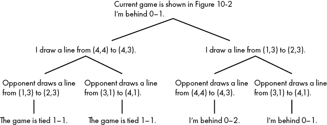
Figure 10-3: A tree of some possible continuations of our game
We start at the top of the tree, considering the current situation: we’re behind 0–1 and it’s our turn to move. One move we consider is the move in the left branch: drawing a line from (4,4) to (4,3). This move will complete a square and give us one point. No matter what move our opponent makes (see the possibilities listed in the two branches in the bottom left of Figure 10-3), the game will be tied after our opponent’s next move. By contrast, if we use our current turn to draw a line from (1,3) to (2,3), as described in Figure 10-3’s right branch, our opponent then has a choice between drawing a line from (4,4) to (4,3) and completing a square and earning a point, or drawing another line like one connecting (3,1) and (4,1), and leaving the score at 0–1.
Considering these possibilities, within two moves the game could be at any of three different scores: 1–1, 0–2, or 0–1. In this tree, it’s clear that we should choose the left branch, because every possibility that grows from that branch leads to a better score for us than do the possibilities growing from the right branch. This style of reasoning is the essence of how our AI will decide on the best move. It will build a game tree, check the outcomes at all terminal nodes of the game tree, and then use simple recursive reasoning to decide what move to make, in light of the possible futures that decision will open up.
You probably noticed that the game tree in Figure 10-3 is woefully incomplete. It appears that there are only two possible moves (the left branch and the right branch), and that after each of those possible moves, our opponent has only two possible moves. Of course, this is incorrect; there are many choices available to both players. Remember that they can connect any two adjacent points in the lattice. The true game tree representing this moment in our game would have many branches, one for each possible move for each player. This is true at every level of the tree: not only do I have many moves to choose from, but so does my opponent, and each of those moves will have its own branch at every point in the tree where it’s playable. Only near the end of the game, when nearly all the line segments have already been drawn, will the number of possible moves shrink to two and one. We didn’t draw every branch of the game tree in Figure 10-3, because there’s not enough space on the page—we only had space to include a couple of moves, just to illustrate the idea of the game tree and our thought process.
You can imagine a game tree extending to any possible depth—we should consider not only our move and the opponent’s response, but also our response to that response, and our opponent’s response to that response, and so on as far as we care to continue the tree-building.
Building Our Tree
The game trees we’re building here are different in important ways from the decision trees of Chapter 9. The most important difference is the goal: decision trees enable classifications and predictions based on characteristics, while game trees simply describe every possible future. Since the goal is different, so will be the way we build it. Remember that in Chapter 9 we had to select a variable and a split point to decide every branch in the tree. Here, knowing what branches will come next is easy, since there will be exactly one branch for every possible move. All we need to do is generate a list of every possible move in our game. We can do this with a couple of nested loops that consider every possible connection between points in our lattice:
allpossible = []

gamesize = 5

for i in range(1,gamesize + 1):
    for j in range(2,gamesize + 1):
        allpossible.append([(i,j),(i,j - 1)])

for i in range(1,gamesize):
    for j in range(1,gamesize + 1):
        allpossible.append([(i,j),(i + 1,j)])
This snippet starts by defining an empty list, called allpossible, and a gamesize variable, which is the length of each side of our lattice. Then, we have two loops. The first is meant to add vertical moves to our list of possible moves. Notice that for every possible value of i and j, this first loop appends the move represented by [(i,j),(i,j - 1)] to our list of possible moves. This will always be a vertical line. Our second loop is similar, but for every possible combination of i and j, it appends the horizontal move [(i,j),(i + 1,j)] to our list of possible moves. At the end, our allpossible list will be populated with every possible move.
If you think about a game that’s in progress, like the game illustrated in Figure 10-2, you’ll realize that not every move is always possible. If a player has already played a particular move during a game, no player can play that same move again for the rest of the game. We’ll need a way to remove all moves that have already been played from the list of all possible moves, resulting in a list of all possible moves remaining for any particular in-progress game. This is easy enough:
for move in allpossible:
    if move in game:
        allpossible.remove(move)
As you can see, we iterate over every move in our list of possible moves, and if it’s already been played, we remove it from our list. In the end, we have a list of only moves that are possible in this particular game. You can run print(allpossible) to see all of these moves and check that they’re correct.
Now that we have a list of every possible move, we can construct the game tree. We’ll record a game tree as a nested list of moves. Remember that each move can be recorded as a list of ordered pairs, like [(4,4),(4,3)], the first move in the left branch of Figure 10-3. If we wanted to express a tree that consisted of only the top two moves in Figure 10-3, we could write it as follows:
simple_tree = [[(4,4),(4,3)],[(1,3),(2,3)]]This tree contains only two moves: the ones we’re considering playing in the current state of the game in Figure 10-3. If we want to include the opponent’s potential responses, we’ll have to add another layer of nesting. We do this by putting each move in a list together with its children, the moves that branch out from the original move. Let’s start by adding empty lists representing a move’s children:
simple_tree_with_children = [[[(4,4),(4,3)],[]],[[(1,3),(2,3)],[]]]Take a moment to make sure you see all the nesting we’ve done. Each move is a list itself, as well as the first element of a list that will also contain the list’s children. Then, all of those lists together are stored in a master list that is our full tree.
We can express the entire game tree from Figure 10-3, including the opponent’s responses, with this nested list structure:
full_tree = [[[(4,4),(4,3)],[[(1,3),(2,3)],[(3,1),(4,1)]]],[[(1,3),(2,3)],[[(4,4),(4,3)],[(3,1),(4,1)]]]]The square brackets quickly get unwieldy, but we need the nested structure so we can correctly keep track of which moves are which moves’ children.
Instead of writing out game trees manually, we can build a function that will create them for us. It will take our list of possible moves as an input and then append each move to the tree (Listing 10-4).
def generate_tree(possible_moves,depth,maxdepth):
    tree = []
    for move in possible_moves:
        move_profile = [move]
        if depth < maxdepth:
            possible_moves2 = possible_moves.copy()
            possible_moves2.remove(move)
            move_profile.append(generate_tree(possible_moves2,depth + 1,maxdepth))
        tree.append(move_profile)
    return(tree)
Listing 10-4: A function that creates a game tree of a specified depth
This function, generate_tree(), starts out by defining an empty list called tree. Then, it iterates over every possible move. For each move, it creates a move_profile. At first, the move_profile consists only of the move itself. But for branches that are not yet at the lowest depth of the tree, we need to add those moves’ children. We add children recursively: we call the generate_tree() function again, but now we have removed one move from the possible_moves list. Finally, we append the move_profile list to the tree.
We can call this function simply, with a couple of lines:
allpossible = [[(4,4),(4,3)],[(4,1),(5,1)]]
thetree = generate_tree(allpossible,0,1)
print(thetree)
When we run this, we see the following tree:
[[[(4, 4), (4, 3)], [[[(4, 1), (5, 1)]]]], [[(4, 1), (5, 1)], [[[(4, 4), (4, 3)]]]]]Next, we’ll make two additions to make our tree more useful: the first records the game score along with the moves, and the second appends a blank list to keep a place for children (Listing 10-5).
def generate_tree(possible_moves,depth,maxdepth,game_so_far):
    tree = []
    for move in possible_moves:
        move_profile = [move]
        game2 = game_so_far.copy()
        game2.append(move)
        move_profile.append(score(game2))
        if depth < maxdepth:
            possible_moves2 = possible_moves.copy()
            possible_moves2.remove(move)
            move_profile.append(generate_tree(possible_moves2,depth + 1,maxdepth,game2))
        else:
            move_profile.append([])
        tree.append(move_profile)
    return(tree)
Listing 10-5: A function that generates a game tree, including child moves and game scores
We can call this again as follows:
allpossible = [[(4,4),(4,3)],[(4,1),(5,1)]]
thetree = generate_tree(allpossible,0,1,[])
print(thetree)
We see the following results:
[[[(4, 4), (4, 3)], [0, 0], [[[(4, 1), (5, 1)], [0, 0], []]]], [[(4, 1), (5, 1)], [0, 0], [[[(4, 4), (4, 3)], [0, 0], []]]]]You can see that each entry in this tree is a full move profile, consisting of a move (like [(4,4),(4,3)]), a score (like [0,0]), and a (sometimes empty) list of children.
Winning a Game
We’re finally ready to create a function that can play dots and boxes well. Before we write the code, let’s consider the principles behind it. Specifically, how is it that we, as humans, play dots and boxes well? More generally, how is it that we go about winning any strategic game (like chess or tic-tac-toe)? Every game has unique rules and features, but there’s a general way to choose a winning strategy based on an analysis of the game tree.
The algorithm we’ll use for choosing a winning strategy is called minimax (a combination of the words minimum and maximum), so called because while we’re trying to maximize our score in the game, our opponent is trying to minimize our score. The constant fight between our maximization and our opponent’s minimization is what we have to strategically consider as we’re choosing the right move.
Let’s look closely at the simple game tree in Figure 10-3. In theory, a game tree can grow to be enormous, with a huge depth and many branches at each depth. But any game tree, big or small, consists of the same components: a lot of little nested branches.
At the point we’re considering in Figure 10-3, we have two choices. Figure 10-4 shows them.
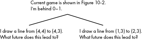
Figure 10-4: Considering which of two moves to choose
Our goal is to maximize our score. To decide between these two moves, we need to know what they will lead to, what future each move brings to pass. To know that, we need to travel farther down the game tree and look at all the possible consequences. Let’s start with the move on the right (Figure 10-5).
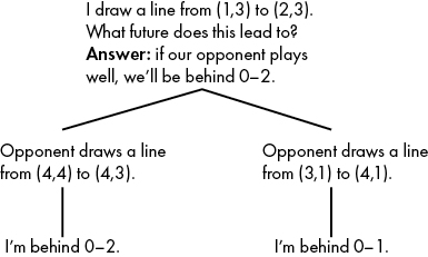
Figure 10-5: Assuming that an opponent will try to minimize your score, you can find what future you expect a move to lead to.
This move could bring about either of two possible futures: we could be behind 0–1 at the end of our tree, or we could be behind 0–2. If our opponent is playing well, they will want to maximize their own score, which is the same as minimizing our score. If our opponent wants to minimize our score, they’ll choose the move that will put us behind 0–2. By contrast, consider our other option, the left branch of Figure 10-5, whose possible futures we consider in Figure 10-6.
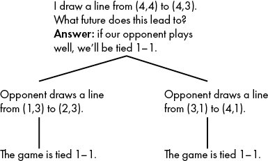
Figure 10-6: No matter what the opponent’s choice, we expect the same outcome.
In this case, both of our opponent’s choices lead to a score of 1–1. Again assuming that our opponent will be acting to minimize our score, we say that this move leads to a future of the game being tied 1–1.
Now we know what future will be brought about by the two moves. Figure 10-7 notes these futures in an updated version of Figure 10-4.
Because we know exactly what future to expect from each of our two moves, we can do a maximization: the move that leads to the maximum, the best score, is the move on the left, so we choose that one.
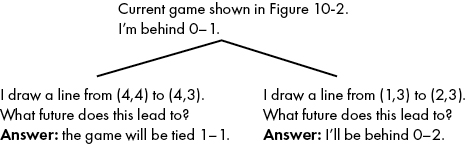
Figure 10-7: Using Figures 10-5 and 10-6, we can reason about the futures that each move will lead to and then compare them.
The reasoning process we just went through is known as the minimax algorithm. Our decision in the present is about maximizing our score. But in order to maximize our score, we have to consider all the ways that our opponent will try to minimize our score. So the best choice is a maximum of minima.
Note that minimax goes through time in reverse. The game proceeds forward in time, from the present to the future. But in a way, the minimax algorithm proceeds backward in time, because we consider the scores of possible far futures first and then work our way back to the present to find the current choice that will lead to the best future. In the context of our game tree, the minimax code starts at the top of the tree. It calls itself recursively on each of its child branches. The child branches, in turn, call minimax recursively on their own child branches. This recursive calling continues all the way to the terminal nodes, where, instead of calling minimax again, we calculate the game score for each node. So we’re calculating the game score for the terminal nodes first; we’re starting our game score calculations in the far future. These scores are then passed back to their parent nodes so that the parent nodes can calculate the best moves and corresponding score for their part of the game. These scores and moves are passed back up through the game tree until arriving back at the very top, the parent node, which represents the present.
Listing 10-6 has a function that accomplishes minimax.
import numpy as np
def minimax(max_or_min,tree):
    allscores = []
    for move_profile in tree:
        if move_profile[2] == []:
            allscores.append(move_profile[1][0] - move_profile[1][1])
        else:
            move,score=minimax((-1) * max_or_min,move_profile[2])
            allscores.append(score)
    newlist = [score * max_or_min for score in allscores]
    bestscore = max(newlist)
    bestmove = np.argmax(newlist)
    return(bestmove,max_or_min * bestscore)
Listing 10-6: A function that uses minimax to find the best move in a game tree
Our minimax() function is relatively short. Most of it is a for loop that iterates over every move profile in our tree. If the move profile has no child moves, then we calculate the score associated with that move as the difference between our squares and our opponent’s squares. If the move profile does have child moves, then we call minimax() on each child to get the score associated with each move. Then all we need to do is find the move associated with the maximum score.
We can call our minimax() function to find the best move to play in any turn in any in-progress game. Let’s make sure everything is defined correctly before we call minimax(). First, let’s define the game, and get all possible moves, using exactly the same code we used before:
allpossible = []

game = [[(1,2),(1,1)],[(3,3),(4,3)],[(1,5),(2,5)],[(1,2),(2,2)],[(2,2),(2,1)],[(1,1),(2,1)],[(3,4),(3,3)],[(3,4),(4,4)]]

gamesize = 5

for i in range(1,gamesize + 1):
    for j in range(2,gamesize + 1):
        allpossible.append([(i,j),(i,j - 1)])

for i in range(1,gamesize):
    for j in range(1,gamesize + 1):
        allpossible.append([(i,j),(i + 1,j)])

for move in allpossible:
    if move in game:
        allpossible.remove(move)
Next, we’ll generate a complete game tree that extends to a depth of three levels:
thetree = generate_tree(allpossible,0,3,game)Now that we have our game tree, we can call our minimax() function:
move,score = minimax(1,thetree)And finally, we can check the best move as follows:
print(thetree[move][0])We see that the best move is [(4, 4), (4, 3)], the move that completes a square and earns us a point. Our AI can play dots and boxes, and choose the best moves! You can try other game board sizes, or different game scenarios, or different tree depths, and check whether our implementation of the minimax algorithm is able to perform well. In a sequel to this book, we’ll discuss how to ensure that your AI doesn’t become simultaneously self-aware and evil and decide to overthrow humanity.
Adding Enhancements
Now that you can perform minimax, you can use it for any game you happen to be playing. Or you can apply it to life decisions, thinking through the future and maximizing every minimum possibility. (The structure of the minimax algorithm will be the same for any competitive scenario, but in order to use our minimax code for a different game, we would have to write new code for the generation of the game tree, the enumeration of every possible move, and the calculation of game scores.)
The AI we’ve built here has very modest capabilities. It’s only able to play one game, with one simple version of the rules. Depending on what processor you use to run this code, it can probably look only a few moves forward without taking an unreasonable amount of time (a few minutes or more) for each decision. It’s natural to want to enhance our AI to make it better.
One thing we’ll definitely want to improve is our AI’s speed. It’s slow because of the large size of the game trees it has to work through. One of the main ways to improve the performance of minimax is by pruning the game tree. Pruning, as you might remember from Chapter 9, is exactly what it sounds like: we remove branches from the tree if we consider them exceptionally poor or if they represent a duplicate of another branch. Pruning is not trivial to implement and requires learning yet more algorithms to do it well. One example is the alpha–beta pruning algorithm, which will stop checking particular sub-branches if they are certainly worse than sub-branches elsewhere in the tree.
Another natural improvement to our AI would be to enable it to work with different rules or different games. For example, a commonly used rule in dots and boxes is that after earning a point, a player gets to draw another line. Sometimes this results in a cascade, in which one player completes many boxes in a row in a single turn. This simple change, which was called “make it, take it” on my elementary school playground, changes the game’s strategic considerations and will require some changes to our code. You can also try to implement an AI that plays dots and boxes on a lattice that has a cross shape or some other exotic shape that could influence strategy. The beauty of minimax is that it doesn’t require subtle strategic understanding; it requires only an ability to look ahead, and that’s why a coder who isn’t good at chess can write an implementation of minimax that can beat them at chess.
There are some powerful methods that go beyond the scope of this chapter that can improve the performance of computer AI. These methods include reinforcement learning (where a chess program, for example, plays against itself to get better), Monte Carlo methods (where a shogi program generates random future shogi games to help understand possibilities), and neural networks (where a tic-tac-toe program predicts what its opponent will do using a machine learning method similar to what we discussed in Chapter 9). These methods are powerful and remarkable, but they mostly just make our tree search and minimax algorithms more efficient; tree search and minimax remain the humble workhorse core of strategic AI.
Summary
In this chapter, we discussed artificial intelligence. It’s a term surrounded by hype, but when you see that it takes only about a dozen lines to write a minimax() function, AI suddenly doesn’t seem so mysterious and intimidating. But of course, to prepare to write those lines, we had to learn the game rules, draw the game board, construct game trees, and configure our minimax() function to calculate game outcomes correctly. Not to mention the rest of the journey of this book, in which we carefully constructed algorithms that prepared us to think algorithmically and to write this function when we needed it.
The next chapter suggests next steps for ambitious algorithmicists who want to continue their journey to the edges of the world of algorithms and push out to further frontiers.