11
ANIMATIONS, SIMULATIONS, AND THE TIME LOOP

The same way vector images visualize static problems, animations help us build visual intuition for dynamic problems. A single image can show us only how things are at a specific point in time. When the properties of a system change over time, we’ll need an animation to get the complete story.

Much like a static analysis presents a system in a moment, a simulation presents the evolution of a system over time. Animations are a good way of presenting the results of this evolution. There are two good reasons for engineers to simulate dynamic systems: it’s a great exercise to solidify your understanding of these systems, and it’s quite fun.

In this chapter, we’ll start exploring the engaging world of animations, starting with a few definitions. We’ll then learn how to make drawings move across the canvas. We’ll use Tkinter’s canvas and, more importantly, our CanvasDrawing wrapper class.

Defining Terms

Let’s define a few of the terms we’ll be using in this section.

What Is an Animation?

An animation is the sensation of motion generated by a rapid succession of images. Because the computer draws these images to the screen extremely quickly, our eyes perceive motion.

We’ll make animations by drawing something to the canvas, clearing it, and then drawing something else. Each drawing, which remains on the screen for a fraction of a second, is called a frame.

Take, for example, Figure 11-1, which depicts each frame of an animation: a triangle moving right.

Figure 11-1: The animation frames of a triangle

Each of the four frames in the animation has the triangle in a slightly different position. If we draw them on the canvas, one after the other, clearing the previous drawing, the triangle will appear to move.

Simple, isn’t it? We’ll build our first animation in this chapter soon, but first let’s define the terms system and simulation, as they’ll appear frequently in our discussion.

What Is a System?

The word system, in our context, refers to whatever we’re drawing to the canvas in an animation. It consists of a group of objects subject to some physical laws and interacting with one another. We’ll use these laws to derive a mathematical model, often in the form of a system of differential equations. We’ll resolve these equations using numerical methods, which yield the values that describe the system at discrete points in time. These values might be the system’s position or velocity.

Now let’s take a look at an example of a system and derive its equation. Let’s suppose we have a body with mass m subject to an external force that is a function of time, . Figure 11-2 depicts a free body diagram. There, you can see the external force and its weight force applied, where is gravity’s acceleration vector.

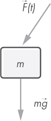
Figure 11-2: A mass subject to external force

Using Newton’s second law and denoting the position vector of the body by , we get the following:

Solving for the acceleration ,

The previous vector equation can be broken down into its two scalar components:

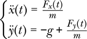
These two equations express the acceleration of the body function of time. To simulate this simple system, we’d need to obtain a new value for the acceleration, velocity, and position of the body for each frame of the animation. We’ll see what this means in a minute.

What Is a Simulation?

A simulation is the study of the evolution of a system whose behavior is mathematically described. Simulations harness the computation power of modern central processing units (CPUs) to understand how a given system would behave under real conditions.

Computer simulations are in general cheaper and simpler to set up than real-world experiments, so they’re used to study and predict the behavior of many engineering designs.

Take the system whose equations we derived in the previous section. Given an expression of the external force with respect to time like

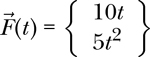
and the mass for the body is said to be m = 5kg, the acceleration equations become the following.

These scalar equations give us the acceleration components for the body at every moment in time. Since the equations are simple, we can integrate them to obtain the expression of the velocity components,

where Ẋ₀ and Ẏ₀ are the components of the initial velocity: the velocity at time t = 0. We know the velocity of the mass for every moment in time. If we want to animate the movement of the mass, we need an expression for the position, which we can obtain by integrating the velocity equations,

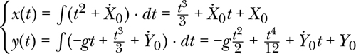
where X₀ and Y₀ are the initial position components for the mass. We can now create an animation to understand how the body moves under the effect of the external force by simply creating a sequence of time values, obtaining the position for each of them, and then drawing a rectangle to the screen at that position.

The differential equations relating how the acceleration of the system varies with respect to time for this example were straightforward, which allowed us to obtain an analytic solution using integration. We usually don’t get an analytic solution for the system under simulation, so we tend to resort to numerical methods.

The analytic solution is the exact solution, whereas a numerical solution is obtained using computer algorithms that look for an approximation of the solution. A common numerical method, although not the most precise, is Euler’s method.

Drawing the simulation in real time means we need to solve the equations as often as we draw frames. For example, if we want to simulate at a rate of 50 frames per second (fps), then we need to both draw the frames and solve the equations 50 times per second.

At 50 fps, the time between frames is 20 milliseconds. Taking into account the fact that your computer requires some of those milliseconds to redraw the screen with the current frame, we’re left with little time for the math.

Simulations can also be computed ahead of time and later played back. This way solving the equations can take as long as required; the animation takes place only when all frames are ready.

Video game engines use real-time simulations as they need to simulate the world around the player as they interact with it, something that can’t be determined ahead of time. These engines tend to trade accuracy for speed; their results are not physically accurate but look realistic to the naked eye.

Complex engineering systems require an ahead-of-time simulation since the governing equations for these problems are complex and require a much more exact solution.

What Is the Time Loop?

Real-time simulations happen inside a loop, which we’ll refer to as the time loop or main loop. This loop executes as many times per second as frames are drawn to the screen. Here’s some pseudocode showing what a time loop might look like:

while current_time < end_time:
    solve_system_equations()
    draw_system()
    sleep(time_delta - time_taken)
    current_time += time_delta

To make the animations look smooth, we want a steady frame rate. This means the drawing phase of the simulation should take place at evenly spaced points in time. (While not strictly necessary, there are techniques to adapt the frame rate to the processor and GPU’s throughput, but we won’t be getting that advanced in this book.)

The time elapsed between consecutive frames is referred to as the time delta, or δt; it’s inversely proportional to the frame rate (fps) and typically measured in seconds or milliseconds: . As a consequence, everything happening in our time loop should take less than a single time delta to complete.

The first step in the loop is solving the equations to figure out how the system has evolved during the elapsed time delta. Then, we draw the system’s new configuration to the screen. We need to measure the time taken so far in the loop and store the result in the time_taken variable.

At this point, the program is paused or put to sleep until an entire time delta has elapsed. The time we sleep can be figured out by subtracting time _taken from time_delta. The last step before ending the loop is to advance the current time by a time delta; the loop then starts over again. Figure 11-3 shows the time line with the events in the time loop drawn.

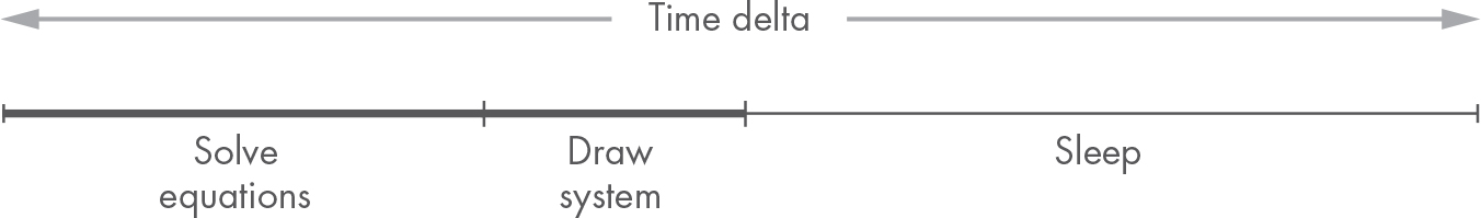
Figure 11-3: The time loop events

Now that we have those definitions out of the way, let’s implement a time loop and start animating.

Our First Animation

At the beginning of the chapter, we explained how we can achieve the sensation of motion by drawing something many times per second. The time loop is in charge of keeping these drawings at a steady rate. Let’s implement our first time loop.

Setup

We’ll start by creating a new file where we can experiment. In the simulation package, create a new file and name it hello_motion.py. Enter the code in Listing 11-1.

  import time
  from tkinter import Tk, Canvas

  tk = Tk()
  tk.title("Hello Motion")

  canvas = Canvas(tk, width=600, height=600)
  canvas.grid(row=0, column=0)

  frame_rate_s = 1.0 / 30.0
  frame_count = 1
  max_frames = 100


  def update_system():
      pass


  def redraw():
      pass


➊ while frame_count <= max_frames:
       update_start = time.time()
➋ update_system()
    ➌ redraw()
    ➍ tk.update()
       update_end = time.time()

    ➎ elapsed_s = update_end - update_start
       remaining_time_s = frame_rate_s - elapsed_s

       if remaining_time_s > 0:
        ➏ time.sleep(remaining_time_s)
      frame_count += 1

  tk.mainloop()

Listing 11-1: The hello_motion.py file

In the code in Listing 11-1, we start by creating a 600 × 600–pixel canvas and adding it to the grid of the main window. Then we initialize some variables: frame_rate_s holds the time between two consecutive frames, in seconds; frame_count is the count of how many frames have already been drawn; and max_frames is the number of total frames we’ll draw.

Then comes the time loop ➊, which executes max_frames times at a rate of frame_rate_s, at least in principle (as you’ll see in a minute). Note that we chose to limit the simulation using a maximum number of frames, but we could also limit it by time, that is, keep running the loop until a given amount of time has elapsed, just like we did in the pseudocode shown earlier. Both approaches work fine.

In the loop we start by storing the current time in update_start. After the updates to the system and the drawing have taken place, we store the time again, this time in update_end. The time elapsed is then computed by subtracting update_start from update_end and stored in elapsed_s ➎. We use this quantity to calculate how long the loop needs to sleep to keep the frame rate steady, subtracting elapsed_s from frame_rate_s. That amount is stored in remaining_time_s, and if it’s greater than zero, we sleep the loop ➏.

If remaining_time_s is less than zero, the loop took longer than the frame rate, meaning it can’t keep up with the rhythm we imposed on it. If this happens often, the time loop will become unsteady, and animations may look chunky, in which case it’s better to simply reduce the frame rate.

The magic happens (or will happen, to be more precise) in update _system ➋ and redraw ➌, which we call in the loop to update and redraw the system. Here’s where we’ll soon be writing our drawing code. The pass statement is used in Python as a placeholder: it doesn’t do anything, but it allows us to have, for example, a valid function body.

There’s also a call to update from main window tk ➍, which tells Tkinter to run the main loop until all pending events have been processed. This is necessary to force Tkinter to look for the events that may trigger changes in the user interface widgets, including our canvas.

You can run the file now; you’ll see an empty window apparently doing nothing, but it’s actually running the loop max_frames times.

Adding a Frame Count Label

Let’s add a label under the canvas to let us know the current frame being drawn to the canvas and the total number of frames. We can update its value in update. First, add Label to the tkinter imports:

from tkinter import Tk, Canvas, StringVar, Label

Then, under the definition of the canvas, add the label (Listing 11-2).

label = StringVar()
label.set('Frame ? of ?')
Label(tk, textvariable=label).grid(row=1, column=0)

Listing 11-2: Adding a label to the window

Finally, update the label’s text in update by setting the value of its text variable, label (Listing 11-3).

def update():
    label.set(f'Frame {frame_count} of {max_frames}')

Listing 11-3: Updating the label’s text

Try to run the file now. The canvas is still blank, but the label below it now displays the current frame. Your program should look like Figure 11-4: a blank window with a frame count going from 1 to 100.

Figure 11-4: The frame count label

Just for reference, your code at this stage should look like Listing 11-4.

import time
from tkinter import Tk, Canvas, StringVar, Label

tk = Tk()
tk.title("Hello Motion")

canvas = Canvas(tk, width=600, height=600)
canvas.grid(row=0, column=0)

label = StringVar()
label.set('Frame ? of ?')
Label(tk, textvariable=label).grid(row=1, column=0)

frame_rate_s = 1.0 / 30.0
frame_count = 1
max_frames = 100


def update_system():
    pass


def redraw():
    label.set(f'Frame {frame_count} of {max_frames}')


while frame_count <= max_frames:
    update_start = time.time()
    update_system()
    redraw()
    tk.update()
    update_end = time.time()

    elapsed_s = update_end - update_start
    remaining_time_s = frame_rate_s - elapsed_s

    if remaining_time_s > 0:
        time.sleep(remaining_time_s)

    frame_count += 1

tk.mainloop()

Listing 11-4: Hello canvas with label

To have anything drawn on the canvas, we need to have a system. Let’s first take a look at how to add and update a system to our simulation.

Updating the System

For this example, we’ll keep it simple and draw a circle whose center is always at the center of the canvas, point (300, 300). Its radius will grow, starting with a value of zero. When the radius grows larger than the canvas and is no longer visible, we’ll set it back to zero. This will generate a psychedelic tunnel-like effect.

We can represent our “system” with an instance of our Circle class. Since we’ll be drawing the circle to the canvas, let’s also create an instance of Canvas Drawing, using an identity affine transformation. Under the definition of variables frame_rate_s, frame_count, and max_frames, add the following:

transform = AffineTransform(sx=1, sy=1, tx=0, ty=0, shx=0, shy=0)
drawing = CanvasDrawing(canvas, transform)
circle = Circle(Point(300, 300), 0)

Don’t forget to include the needed imports:

from geom2d import Point, Circle, AffineTransform
from graphic.simulation.draw import CanvasDrawing

We need to update the value of the radius every frame in update_system so that when redraw does its thing, the circle gets drawn with the updated value for the radius. In update_system, enter the code in Listing 11-5.

def update_system():
    circle.radius = (circle.radius + 15) % 450
    tk.update()

Listing 11-5: Updating the circle’s radius

The value for the radius is updated by adding 15 to the current value. Using the modulo operator (%), whenever the radius becomes greater than 450, the value wraps around and goes back to zero.

You’ve probably realized that we mutated the circle’s radius property instead of creating a new circle with the value for the new radius; it’s the first time in the book we mutate the properties of our geometric primitives. The reason is that, for simulations, maintaining the throughput of the loop is crucial, and creating a new instance of the system for each frame would have a high performance impact.

We now have the system defined in each of the frames: a circle whose center point is kept centered in the window while the radius gradually increases in size. Let’s draw it to the screen!

Creating Motion

To create the effect of motion, the canvas has to be cleared and the system redrawn in each and every frame. Before redraw is invoked in the main loop, update_system has already updated the circle. In redraw, we simply need to clear whatever is drawn on the canvas and draw the circle again. Update redraw using the code in Listing 11-6.

def redraw():
    label.set(f'Frame {frame_count} of {max_frames}')
    drawing.clear_drawing()
    drawing.draw_circle(circle, 50)

Listing 11-6: Redrawing the circle every frame

You’ve probably been waiting for this grand moment for the whole chapter, so go ahead and execute the file. You should see a circle growing in size until it disappears from the screen and then starting over again.

Just for your reference, at this point, your hello_motion.py code should look like Listing 11-7.

import time
from tkinter import Tk, Canvas, StringVar, Label

from geom2d import Point, AffineTransform, Circle
from graphic.simulation import CanvasDrawing

tk = Tk()
tk.title("Hello Motion")

canvas = Canvas(tk, width=600, height=600)
canvas.grid(row=0, column=0)

label = StringVar()
label.set('Frame ? of ?')
Label(tk, textvariable=label).grid(row=1, column=0)

frame_rate_s = 1.0 / 30.0
frame_count = 1
max_frames = 100

transform = AffineTransform(sx=1, sy=1, tx=0, ty=0, shx=0, shy=0)
drawing = CanvasDrawing(canvas, transform)
circle = Circle(Point(300, 300), 0)


def update_system():
    circle.radius = (circle.radius + 15) % 450
    tk.update()


def redraw():
    label.set(f'Frame {frame_count} of {max_frames}')
    drawing.clear_drawing()
    drawing.draw_circle(circle, 50)


while frame_count <= max_frames:
    update_start = time.time()
    update_system()
    redraw()
    tk.update()
    update_end = time.time()

    elapsed_s = update_end - update_start
    remaining_time_s = frame_rate_s - elapsed_s

    if remaining_time_s > 0:
        time.sleep(remaining_time_s)

    frame_count += 1

tk.mainloop()

Listing 11-7: Resulting simulation

Note that before drawing anything, the redraw function clears the canvas. Can you guess what would happen if we forgot to do so? Comment that line out and run the simulation.

def redraw():
    label.set(f'Frame {frame_count} of {max_frames}')
    # drawing.clear_drawing()
    drawing.draw_circle(circle, 50)

All circles drawn should remain on the canvas, as you see in Figure 11-5.

We’ve drawn our first animation on the canvas, and it looks fantastic. If we were to write another, though, we’d have to copy and paste the code for the main loop. To avoid this needless duplication, let’s move the main loop code into a function that can be easily reused.

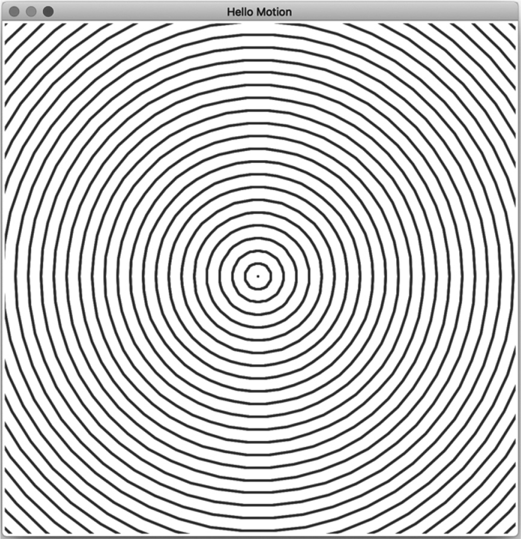
Figure 11-5: What it’d look like if we forgot to clean the canvas

Abstracting the Main Loop Function

The main loop we just wrote had a fair amount of logic that will be the same for all simulations. Copying and pasting this code over and over again would not only be bad practice, but if we found an improvement or wanted to make a change to our implementation, we’d need to edit the code of all our simulations. We don’t want to duplicate knowledge: we should define the logic for a main simulation loop in just one place.

To implement a generic version of the main loop, we need to do an abstraction exercise. Let’s ask ourselves the following questions regarding the implementation of the main loop: Is there something that’s never going to change in it, and is there anything simulation-specific? The while loop, the order of the operations inside of it, and the time calculations are the same for every simulation. Conversely, there are three pieces of logic that vary from simulation to simulation, namely, the decision that keeps the loop running, the updating, and the drawing.

If we encapsulate those in functions that the simulations implement, they can be passed to our main loop abstraction. The main loop we implement only needs to care about the timing, that is, trying to keep the frame rate stable.

Create a new file named loop.py in the simulation package. Enter the code in Listing 11-8.

import time


def main_loop(
        update_fn,
        redraw_fn,
        should_continue_fn,
        frame_rate_s=0.03
):
    frame = 1
    time_s = 0
    last_elapsed_s = frame_rate_s

 ➊ while should_continue_fn(frame, time_s):
        update_start = time.time()
     ➋ update_fn(last_elapsed_s, time_s, frame)
     ➌ redraw_fn()
        update_end = time.time()

        elapsed_s = update_end - update_start
        remaining_time_s = frame_rate_s - elapsed_s

        if remaining_time_s > 0:
            time.sleep(remaining_time_s)
            last_elapsed_s = frame_rate_s
        else:
            last_elapsed_s = elapsed_s


        frame += 1
        time_s += last_elapsed_s

Listing 11-8: Simulation’s main loop function

The first thing you should notice is that three of the arguments to the main_loop function are also functions: update_fn, redraw_fn, and should_continue _fn. These functions contain the logic that’s simulation-specific, so our main loop simply needs to call them as needed.

The main_loop function starts by declaring three variables: frame, which holds the current frame index; time_s, which holds the total time elapsed; and last_elapsed_s, which holds the number of seconds it took the last frame to complete. The condition to keep the loop running is now delegated to the should_continue_fn function ➊. The loop will continue as long as this function returns true. It accepts two arguments: the frame count and the total time elapsed in seconds. If you recall, most of our simulations will be limited by one of these values, so we pass them to the function so that it has the information required to decide whether the loop should keep running.

Next, the update_fn function ➋ updates the system under simulation and the user interface. This function receives three parameters: the time elapsed since the last frame, last_elapsed_s; the total elapsed time for the simulation, time_s; and the current frame number, frame. As we’ll see later in the book, when we introduce physics to our simulations, the amount of time elapsed since the last frame is an important piece of data. Lastly comes redraw_fn ➌, which draws the system to the screen.

Thanks to our abstraction of the simulation’s main loop, we won’t need to write this logic anymore. Let’s try to refactor our simulation from the previous section using this definition of the main loop.

Refactoring Our Simulation

Now that we’ve created an abstraction of the main loop, let’s take a look at how our simulation could be refactored to include the main loop function.

Create a new file named hello_motion_refactor.py and enter the code from Listing 11-9. You may want to copy and paste the first lines from hello_motion.py, those that define the UI. Note that to make the code a bit shorter, I’ve removed the frame count label from the UI.

from tkinter import Tk, Canvas

from geom2d import Point, Circle, AffineTransform
from graphic.simulation.draw import CanvasDrawing
from graphic.simulation.loop import main_loop

tk = Tk()
tk.title("Hello Motion")

canvas = Canvas(tk, width=600, height=600)
canvas.grid(row=0, column=0)

max_frames = 100

transform = AffineTransform(sx=1, sy=1, tx=0, ty=0, shx=0, shy=0)
drawing = CanvasDrawing(canvas, transform)
circle = Circle(Point(300, 300), 0)


def update_system(time_delta_s, time_s, frame):
    circle.radius = (circle.radius + 15) % 450
    tk.update()


def redraw():
    drawing.clear_drawing()
    drawing.draw_circle(circle, 50)


def should_continue(frame, time_s):
    return frame <= max_frames


main_loop(update_system, redraw, should_continue)
tk.mainloop()

Listing 11-9: Refactored version of hello_motion.py

If we go toward the end of the code, we find the call to main_loop. We’re passing in the functions that we previously defined, with the sole difference being that now those functions must declare the proper parameters to match the functions main_loop expects.

This code is much simpler to follow. All the logic to keep a steady frame rate has been moved away to its own function, so we can focus our attention on the simulation itself without needing to deal with those details. Let’s now take some time to play with some of the parameters of the simulation and understand how they affect the final result.

Playing with the Circle Divisions

Remember that the CanvasDrawing class includes an affine transformation as part of its state, and every geometric primitive gets transformed by it before being drawn. Remember also that this is the reason a circle is converted to a generic polygon using a number of divisions high enough to approximate the circumference. The transformation happens in the drawing command; hence, the number of divisions has to be passed in, or else the default of 30 is used.

Going back to function redraw from Listing 11-9,

def redraw():
    drawing.clear_drawing()
    drawing.draw_circle(circle, 50)

you can see we used 50 divisions, but we could have used any other number. Let’s try with 10, for example:

def redraw():
    drawing.clear_drawing()
    drawing.draw_circle(circle, 10)

Rerun the file. Can you see the difference? What about if you try with 6 divisions? Figure 11-6 shows the simulation using 50, 10, and 6 divisions for the circle.

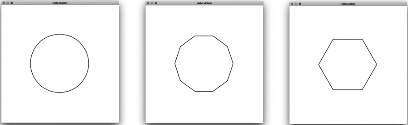
Figure 11-6: Circles drawn using 50, 10, and 6 divisions

After this interesting experiment we can clearly see the influence of the divisions used to approximate a circle. Let’s now experiment with the affine transformation used to transform the geometric primitives before they’re drawn to the canvas.

Playing with the Affine Transformation

The affine transformation applied to the drawing in our simulation is an identity transformation: it keeps points exactly where they are. But we could use this transformation to do something different, such as invert the y-axis so that it points upward, for example. Go back to hello_motion_refactor.py and locate the line where the transformation is defined:

transform = AffineTransform(sx=1, sy=1, tx=0, ty=0, shx=0, shy=0)

Then, edit it so that it inverts the y-axis:

transform = AffineTransform(
    sx=1, sy=-1, tx=0, ty=0, shx=0, shy=0
)

Run the simulation again. What do you see? Just a little rim coming from the top of the canvas, right? What’s happening is that we inverted the y-axis, but the origin of coordinates is still in the upper-left corner; thus, the circle we’re trying to draw is outside the window, as depicted by Figure 11-7.

Figure 11-7: Simulation with the y-axis inverted

We can easily fix this problem by translating the origin of the coordinates all the way down to the lower-left corner of the canvas. Since the canvas height is 600 pixels, we can set the transformation to be as follows:

transform = AffineTransform(
    sx=1, sy=-1, tx=0, ty=600, shx=0, shy=0
)

It may surprise you that the value for the vertical translation is 600 and not – 600, but remember that in the original system of coordinates, the y direction points downward, and this affine transformation refers to that system.

If you prefer, it may be easier to understand the process of obtaining that transformation by concatenating two simpler ones, the first moving the origin downward 600 pixels and the second flipping the y-axis,

>>> t1 = AffineTransform(sx=1, sy=1, tx=0, ty=-600, shx=0, shy=0)
>>> t2 = AffineTransform(sx=1, sy=-1, tx=0, ty=0, shx=0, shy=0)
>>> t1.then(t2).__dict__
{'sx': 1, 'sy': -1, 'tx': 0, 'ty': 600, 'shx': 0, 'shy': 0}

which yields the same transformation, as you can see.

Now, let’s add some shear in the horizontal direction to see how the circle gets deformed. Try the following values for the transformation,

transform = AffineTransform(
    sx=1, sy=-1, tx=150, ty=600, shx=-0.5, shy=0
)

and run the simulation again. You should see a shape similar to that in Figure 11-8.

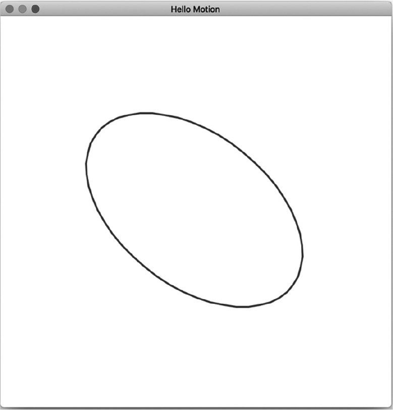
Figure 11-8: A circle drawn using a horizontal shear

Now it’s your turn to play with the values and see whether you can build a better intuition for how the animations, drawings, and transformations are working. You’ve created something beautiful from scratch, so take your time to experiment with it. Try to change the circle primitive using a triangle or a rectangle. You can update the geometric primitive by moving it instead of changing its size. Play around with the affine transformation values and try to reason about how the drawing should look before you actually run the simulation. Use this exercise to reinforce your affine transformation intuition.

Cleaning Up the Module

Let’s do two small refactors to the module to clean it up a bit. First, create a new folder in the simulation package and name it examples. We’ll use it to house all the files that are not part of the simulation and drawing logic, but rather examples we wrote in this chapter. So, basically, move all the files except for draw.py and loop.py there. Your folder structure in simulation should look like this:

    simulation
      |- examples
      |    |- hello_canvas.py
      |    |- hello_motion.py
      |    |- ...
      |
      |- __init__.py
      |- draw.py
      |- loop.py

The second thing we want to do is add both the CanvasDrawing class and the main_loop function to the default exports of the simulation package. Open file __init__.py in simulation and add the following imports:

from .draw import CanvasDrawing
from .loop import main_loop

That’s it! From now on we’ll be able to import both using a shorter syntax.

Summary

In this chapter, we learned about the time loop. The time loop keeps executing while a condition is met, and its main job is to keep the frame rate steady. In this loop two things take place: the updating of the system under simulation and the redrawing of the screen. Those operations are timed so that when they’re done, we know how much more time remains to complete a cycle.

Because the time loop will appear in all of our simulations, we decided to implement it as a function. This function gets passed other functions: one that updates the system, another that draws it to the screen, and a last one that decides whether the simulation is over or not.

In the next chapter, we’ll use this time loop function to animate affine transformations.