
CHAPTER 8
Main Memory
In Chapter 6, we showed how the CPU can be shared by a set of processes. As a result of CPU scheduling, we can improve both the utilization of the CPU and the speed of the computer's response to its users. To realize this increase in performance, however, we must keep several processes in memory—that is, we must share memory.
In this chapter, we discuss various ways to manage memory. The memory-management algorithms vary from a primitive bare-machine approach to paging and segmentation strategies. Each approach has its own advantages and disadvantages. Selection of a memory-management method for a specific system depends on many factors, especially on the hardware design of the system. As we shall see, many algorithms require hardware support, leading many systems to have closely integrated hardware and operating-system memory management.
CHAPTER OBJECTIVES
- To provide a detailed description of various ways of organizing memory hardware.
- To explore various techniques of allocating memory to processes.
- To discuss in detail how paging works in contemporary computer systems.
8.1 Background
As we saw in Chapter 1, memory is central to the operation of a modern computer system. Memory consists of a large array of bytes, each with its own address. The CPU fetches instructions from memory according to the value of the program counter. These instructions may cause additional loading from and storing to specific memory addresses.
A typical instruction-execution cycle, for example, first fetches an instruction from memory. The instruction is then decoded and may cause operands to be fetched from memory. After the instruction has been executed on the operands, results may be stored back in memory. The memory unit sees only a stream of memory addresses; it does not know how they are generated (by the instruction counter, indexing, indirection, literal addresses, and so on) or what they are for (instructions or data). Accordingly, we can ignore how a program generates a memory address. We are interested only in the sequence of memory addresses generated by the running program.
We begin our discussion by covering several issues that are pertinent to managing memory: basic hardware, the binding of symbolic memory addresses to actual physical addresses, and the distinction between logical and physical addresses. We conclude the section with a discussion of dynamic linking and shared libraries.
8.1.1 Basic Hardware
Main memory and the registers built into the processor itself are the only general-purpose storage that the CPU can access directly. There are machine instructions that take memory addresses as arguments, but none that take disk addresses. Therefore, any instructions in execution, and any data being used by the instructions, must be in one of these direct-access storage devices. If the data are not in memory, they must be moved there before the CPU can operate on them.
Registers that are built into the CPU are generally accessible within one cycle of the CPU clock. Most CPUs can decode instructions and perform simple operations on register contents at the rate of one or more operations per clock tick. The same cannot be said of main memory, which is accessed via a transaction on the memory bus. Completing a memory access may take many cycles of the CPU clock. In such cases, the processor normally needs to stall, since it does not have the data required to complete the instruction that it is executing. This situation is intolerable because of the frequency of memory accesses. The remedy is to add fast memory between the CPU and main memory, typically on the CPU chip for fast access. Such a cache was described in Section 1.8.3. To manage a cache built into the CPU, the hardware automatically speeds up memory access without any operating-system control.
Not only are we concerned with the relative speed of accessing physical memory, but we also must ensure correct operation. For proper system operation we must protect the operating system from access by user processes. On multiuser systems, we must additionally protect user processes from one another. This protection must be provided by the hardware because the operating system doesn't usually intervene between the CPU and its memory accesses (because of the resulting performance penalty). Hardware implements this production in several different ways, as we show throughout the chapter. Here, we outline one possible implementation.
We first need to make sure that each process has a separate memory space. Separate per-process memory space protects the processes from each other and is fundamental to having multiple processes loaded in memory for concurrent execution. To separate memory spaces, we need the ability to determine the range of legal addresses that the process may access and to ensure that the process can access only these legal addresses. We can provide this protection by using two registers, usually a base and a limit, as illustrated in Figure 8.1. The base register holds the smallest legal physical memory address; the limit register specifies the size of the range. For example, if the base register holds 300040 and the limit register is 120900, then the program can legally access all addresses from 300040 through 420939 (inclusive).
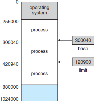
Figure 8.1 A base and a limit register define a logical address space.
Protection of memory space is accomplished by having the CPU hardware compare every address generated in user mode with the registers. Any attempt by a program executing in user mode to access operating-system memory or other users' memory results in a trap to the operating system, which treats the attempt as a fatal error (Figure 8.2). This scheme prevents a user program from (accidentally or deliberately) modifying the code or data structures of either the operating system or other users.
The base and limit registers can be loaded only by the operating system, which uses a special privileged instruction. Since privileged instructions can be executed only in kernel mode, and since only the operating system executes in kernel mode, only the operating system can load the base and limit registers. This scheme allows the operating system to change the value of the registers but prevents user programs from changing the registers' contents.
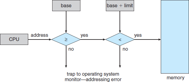
Figure 8.2 Hardware address protection with base and limit registers.
The operating system, executing in kernel mode, is given unrestricted access to both operating-system memory and users' memory. This provision allows the operating system to load users' programs into users' memory, to dump out those programs in case of errors, to access and modify parameters of system calls, to perform I/O to and from user memory, and to provide many other services. Consider, for example, that an operating system for a multiprocessing system must execute context switches, storing the state of one process from the registers into main memory before loading the next process's context from main memory into the registers.
8.1.2 Address Binding
Usually, a program resides on a disk as a binary executable file. To be executed, the program must be brought into memory and placed within a process. Depending on the memory management in use, the process may be moved between disk and memory during its execution. The processes on the disk that are waiting to be brought into memory for execution form the input queue.
The normal single-tasking procedure is to select one of the processes in the input queue and to load that process into memory. As the process is executed, it accesses instructions and data from memory. Eventually, the process terminates, and its memory space is declared available.
Most systems allow a user process to reside in any part of the physical memory. Thus, although the address space of the computer may start at 00000, the first address of the user process need not be 00000. You will see later how a user program actually places a process in physical memory.
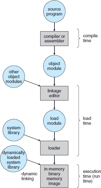
In most cases, a user program goes through several steps—some of which may be optional—before being executed (Figure 8.3). Addresses may be represented in different ways during these steps. Addresses in the source program are generally symbolic (such as the variable count). A compiler typically binds these symbolic addresses to relocatable addresses (such as “14 bytes from the beginning of this module”). The linkage editor or loader in turn binds the relocatable addresses to absolute addresses (such as 74014). Each binding is a mapping from one address space to another.
Classically, the binding of instructions and data to memory addresses can be done at any step along the way:
- Compile time. If you know at compile time where the process will reside in memory, then absolute code can be generated. For example, if you know that a user process will reside starting at location R, then the generated compiler code will start at that location and extend up from there. If, at some later time, the starting location changes, then it will be necessary to recompile this code. The MS-DOS .COM-format programs are bound at compile time.
- Load time. If it is not known at compile time where the process will reside in memory, then the compiler must generate relocatable code. In this case, final binding is delayed until load time. If the starting address changes, we need only reload the user code to incorporate this changed value.
- Execution time. If the process can be moved during its execution from one memory segment to another, then binding must be delayed until run time. Special hardware must be available for this scheme to work, as will be discussed in Section 8.1.3. Most general-purpose operating systems use this method.
A major portion of this chapter is devoted to showing how these various bindings can be implemented effectively in a computer system and to discussing appropriate hardware support.
8.1.3 Logical Versus Physical Address Space
An address generated by the CPU is commonly referred to as a logical address, whereas an address seen by the memory unit—that is, the one loaded into the memory-address register of the memory—is commonly referred to as a physical address.
The compile-time and load-time address-binding methods generate identical logical and physical addresses. However, the execution-time address-binding scheme results in differing logical and physical addresses. In this case, we usually refer to the logical address as a virtual address. We use logical address and virtual address interchangeably in this text. The set of all logical addresses generated by a program is a logical address space. The set of all physical addresses corresponding to these logical addresses is a physical address space. Thus, in the execution-time address-binding scheme, the logical and physical address spaces differ.
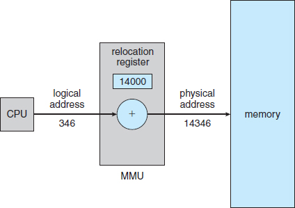
Figure 8.4 Dynamic relocation using a relocation register.
The run-time mapping from virtual to physical addresses is done by a hardware device called the memory-management unit (MMU). We can choose from many different methods to accomplish such mapping, as we discuss in Section 8.3 through Section 8.5. For the time being, we illustrate this mapping with a simple MMU scheme that is a generalization of the base-register scheme described in Section 8.1.1. The base register is now called a relocation register. The value in the relocation register is added to every address generated by a user process at the time the address is sent to memory (see Figure 8.4). For example, if the base is at 14000, then an attempt by the user to address location 0 is dynamically relocated to location 14000; an access to location 346 is mapped to location 14346.
The user program never sees the real physical addresses. The program can create a pointer to location 346, store it in memory, manipulate it, and compare it with other addresses—all as the number 346. Only when it is used as a memory address (in an indirect load or store, perhaps) is it relocated relative to the base register. The user program deals with logical addresses. The memory-mapping hardware converts logical addresses into physical addresses. This form of execution-time binding was discussed in Section 8.1.2. The final location of a referenced memory address is not determined until the reference is made.
We now have two different types of addresses: logical addresses (in the range 0 to max) and physical addresses (in the range R + 0 to R + max for a base value R). The user program generates only logical addresses and thinks that the process runs in locations 0 to max. However, these logical addresses must be mapped to physical addresses before they are used. The concept of a logical address space that is bound to a separate physical address space is central to proper memory management.
8.1.4 Dynamic Loading
In our discussion so far, it has been necessary for the entire program and all data of a process to be in physical memory for the process to execute. The size of a process has thus been limited to the size of physical memory. To obtain better memory-space utilization, we can use dynamic loading. With dynamic loading, a routine is not loaded until it is called. All routines are kept on disk in a relocatable load format. The main program is loaded into memory and is executed. When a routine needs to call another routine, the calling routine first checks to see whether the other routine has been loaded. If it has not, the relocatable linking loader is called to load the desired routine into memory and to update the program's address tables to reflect this change. Then control is passed to the newly loaded routine.
The advantage of dynamic loading is that a routine is loaded only when it is needed. This method is particularly useful when large amounts of code are needed to handle infrequently occurring cases, such as error routines. In this case, although the total program size may be large, the portion that is used (and hence loaded) may be much smaller.
Dynamic loading does not require special support from the operating system. It is the responsibility of the users to design their programs to take advantage of such a method. Operating systems may help the programmer, however, by providing library routines to implement dynamic loading.
8.1.5 Dynamic Linking and Shared Libraries
Dynamically linked libraries are system libraries that are linked to user programs when the programs are run (refer back to Figure 8.3). Some operating systems support only static linking, in which system libraries are treated like any other object module and are combined by the loader into the binary program image. Dynamic linking, in contrast, is similar to dynamic loading. Here, though, linking, rather than loading, is postponed until execution time. This feature is usually used with system libraries, such as language subroutine libraries. Without this facility, each program on a system must include a copy of its language library (or at least the routines referenced by the program) in the executable image. This requirement wastes both disk space and main memory.
With dynamic linking, a stub is included in the image for each library-routine reference. The stub is a small piece of code that indicates how to locate the appropriate memory-resident library routine or how to load the library if the routine is not already present. When the stub is executed, it checks to see whether the needed routine is already in memory. If it is not, the program loads the routine into memory. Either way, the stub replaces itself with the address of the routine and executes the routine. Thus, the next time that particular code segment is reached, the library routine is executed directly, incurring no cost for dynamic linking. Under this scheme, all processes that use a language library execute only one copy of the library code.
This feature can be extended to library updates (such as bug fixes). A library may be replaced by a new version, and all programs that reference the library will automatically use the new version. Without dynamic linking, all such programs would need to be relinked to gain access to the new library. So that programs will not accidentally execute new, incompatible versions of libraries, version information is included in both the program and the library. More than one version of a library may be loaded into memory, and each program uses its version information to decide which copy of the library to use. Versions with minor changes retain the same version number, whereas versions with major changes increment the number. Thus, only programs that are compiled with the new library version are affected by any incompatible changes incorporated in it. Other programs linked before the new library was installed will continue using the older library. This system is also known as shared libraries.
Unlike dynamic loading, dynamic linking and shared libraries generally require help from the operating system. If the processes in memory are protected from one another, then the operating system is the only entity that can check to see whether the needed routine is in another process's memory space or that can allow multiple processes to access the same memory addresses. We elaborate on this concept when we discuss paging in Section 8.5.4.
8.2 Swapping
A process must be in memory to be executed. A process, however, can be swapped temporarily out of memory to a backing store and then brought back into memory for continued execution (Figure 8.5). Swapping makes it possible for the total physical address space of all processes to exceed the real physical memory of the system, thus increasing the degree of multiprogramming in a system.
8.2.1 Standard Swapping
Standard swapping involves moving processes between main memory and a backing store. The backing store is commonly a fast disk. It must be large enough to accommodate copies of all memory images for all users, and it must provide direct access to these memory images. The system maintains a ready queue consisting of all processes whose memory images are on the backing store or in memory and are ready to run. Whenever the CPU scheduler decides to execute a process, it calls the dispatcher. The dispatcher checks to see whether the next process in the queue is in memory. If it is not, and if there is no free memory region, the dispatcher swaps out a process currently in memory and swaps in the desired process. It then reloads registers and transfers control to the selected process.
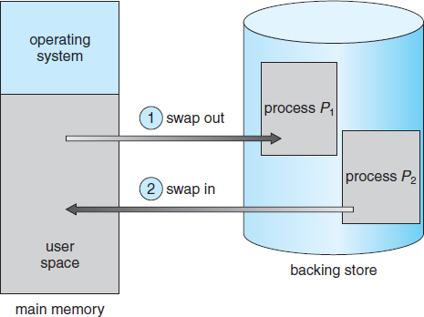
Figure 8.5 Swapping of two processes using a disk as a backing store.
The context-switch time in such a swapping system is fairly high. To get an idea of the context-switch time, let's assume that the user process is 100 MB in size and the backing store is a standard hard disk with a transfer rate of 50 MB per second. The actual transfer of the 100-MB process to or from main memory takes
100 MB/50 MB per second = 2 seconds
The swap time is 200 milliseconds. Since we must swap both out and in, the total swap time is about 4,000 milliseconds. (Here, we are ignoring other disk performance aspects, which we cover in Chapter 10.)
Notice that the major part of the swap time is transfer time. The total transfer time is directly proportional to the amount of memory swapped. If we have a computer system with 4 GB of main memory and a resident operating system taking 1 GB, the maximum size of the user process is 3 GB. However, many user processes may be much smaller than this—say, 100MB. A 100-MB process could be swapped out in 2 seconds, compared with the 60 seconds required for swapping 3 GB. Clearly, it would be useful to know exactly how much memory a user process is using, not simply how much it might be using. Then we would need to swap only what is actually used, reducing swap time. For this method to be effective, the user must keep the system informed of any changes in memory requirements. Thus, a process with dynamic memory requirements will need to issue system calls (request_memory() and release_memory()) to inform the operating system of its changing memory needs.
Swapping is constrained by other factors as well. If we want to swap a process, we must be sure that it is completely idle. Of particular concern is any pending I/O. A process may be waiting for an I/O operation when we want to swap that process to free up memory. However, if the I/O is asynchronously accessing the user memory for I/O buffers, then the process cannot be swapped. Assume that the I/O operation is queued because the device is busy. If we were to swap out process P1 and swap in process P2, the I/O operation might then attempt to use memory that now belongs to process P2. There are two main solutions to this problem: never swap a process with pending I/O, or execute I/O operations only into operating-system buffers. Transfers between operating-system buffers and process memory then occur only when the process is swapped in. Note that this double buffering itself adds overhead. We now need to copy the data again, from kernel memory to user memory, before the user process can access it.
Standard swapping is not used in modern operating systems. It requires too much swapping time and provides too little execution time to be a reasonable memory-management solution. Modified versions of swapping, however, are found on many systems, including UNIX, Linux, and Windows. In one common variation, swapping is normally disabled but will start if the amount of free memory (unused memory available for the operating system or processes to use) falls below a threshold amount. Swapping is halted when the amount of free memory increases. Another variation involves swapping portions of processes—rather than entire processes—to decrease swap time. Typically, these modified forms of swapping work in conjunction with virtual memory, which we cover in Chapter 9.
8.2.2 Swapping on Mobile Systems
Although most operating systems for PCs and servers support some modified version of swapping, mobile systems typically do not support swapping in any form. Mobile devices generally use flash memory rather than more spacious hard disks as their persistent storage. The resulting space constraint is one reason why mobile operating-system designers avoid swapping. Other reasons include the limited number of writes that flash memory can tolerate before it becomes unreliable and the poor throughput between main memory and flash memory in these devices.
Instead of using swapping, when free memory falls below a certain threshold, Apple's iOS asks applications to voluntarily relinquish allocated memory. Read-only data (such as code) are removed from the system and later reloaded from flash memory if necessary. Data that have been modified (such as the stack) are never removed. However, any applications that fail to free up sufficient memory may be terminated by the operating system.
Android does not support swapping and adopts a strategy similar to that used by iOS. It may terminate a process if insufficient free memory is available. However, before terminating a process, Android writes its application state to flash memory so that it can be quickly restarted.
Because of these restrictions, developers for mobile systems must carefully allocate and release memory to ensure that their applications do not use too much memory or suffer from memory leaks. Note that both iOS and Android support paging, so they do have memory-management abilities. We discuss paging later in this chapter.
8.3 Contiguous Memory Allocation
The main memory must accommodate both the operating system and the various user processes. We therefore need to allocate main memory in the most efficient way possible. This section explains one early method, contiguous memory allocation.
The memory is usually divided into two partitions: one for the resident operating system and one for the user processes. We can place the operating system in either low memory or high memory. The major factor affecting this decision is the location of the interrupt vector. Since the interrupt vector is often in low memory, programmers usually place the operating system in low memory as well. Thus, in this text, we discuss only the situation in which the operating system resides in low memory. The development of the other situation is similar.
We usually want several user processes to reside in memory at the same time. We therefore need to consider how to allocate available memory to the processes that are in the input queue waiting to be brought into memory. In contiguous memory allocation, each process is contained in a single section of memory that is contiguous to the section containing the next process.
8.3.1 Memory Protection
Before discussing memory allocation further, we must discuss the issue of memory protection. We can prevent a process from accessing memory it does not own by combining two ideas previously discussed. If we have a system with a relocation register (Section 8.1.3), together with a limit register (Section 8.1.1), we accomplish our goal. The relocation register contains the value of the smallest physical address; the limit register contains the range of logical addresses (for example, relocation = 100040 and limit = 74600). Each logical address must fall within the range specified by the limit register. The MMU maps the logical address dynamically by adding the value in the relocation register. This mapped address is sent to memory (Figure 8.6).
When the CPU scheduler selects a process for execution, the dispatcher loads the relocation and limit registers with the correct values as part of the context switch. Because every address generated by a CPU is checked against these registers, we can protect both the operating system and the other users' programs and data from being modified by this running process.
The relocation-register scheme provides an effective way to allow the operating system's size to change dynamically. This flexibility is desirable in many situations. For example, the operating system contains code and buffer space for device drivers. If a device driver (or other operating-system service) is not commonly used, we do not want to keep the code and data in memory, as we might be able to use that space for other purposes. Such code is sometimes called transient operating-system code; it comes and goes as needed. Thus, using this code changes the size of the operating system during program execution.
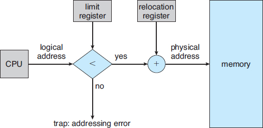
Figure 8.6 Hardware support for relocation and limit registers.
8.3.2 Memory Allocation
Now we are ready to turn to memory allocation. One of the simplest methods for allocating memory is to divide memory into several fixed-sized partitions. Each partition may contain exactly one process. Thus, the degree of multiprogramming is bound by the number of partitions. In this multiple-partition method, when a partition is free, a process is selected from the input queue and is loaded into the free partition. When the process terminates, the partition becomes available for another process. This method was originally used by the IBM OS/360 operating system (called MFT) but is no longer in use. The method described next is a generalization of the fixed-partition scheme (called MVT); it is used primarily in batch environments. Many of the ideas presented here are also applicable to a time-sharing environment in which pure segmentation is used for memory management (Section 8.4).
In the variable-partition scheme, the operating system keeps a table indicating which parts of memory are available and which are occupied. Initially, all memory is available for user processes and is considered one large block of available memory, a hole. Eventually, as you will see, memory contains a set of holes of various sizes.
As processes enter the system, they are put into an input queue. The operating system takes into account the memory requirements of each process and the amount of available memory space in determining which processes are allocated memory. When a process is allocated space, it is loaded into memory, and it can then compete for CPU time. When a process terminates, it releases its memory, which the operating system may then fill with another process from the input queue.
At any given time, then, we have a list of available block sizes and an input queue. The operating system can order the input queue according to a scheduling algorithm. Memory is allocated to processes until, finally, the memory requirements of the next process cannot be satisfied—that is, no available block of memory (or hole) is large enough to hold that process. The operating system can then wait until a large enough block is available, or it can skip down the input queue to see whether the smaller memory requirements of some other process can be met.
In general, as mentioned, the memory blocks available comprise a set of holes of various sizes scattered throughout memory. When a process arrives and needs memory, the system searches the set for a hole that is large enough for this process. If the hole is too large, it is split into two parts. One part is allocated to the arriving process; the other is returned to the set of holes. When a process terminates, it releases its block of memory, which is then placed back in the set of holes. If the new hole is adjacent to other holes, these adjacent holes are merged to form one larger hole. At this point, the system may need to check whether there are processes waiting for memory and whether this newly freed and recombined memory could satisfy the demands of any of these waiting processes.
This procedure is a particular instance of the general dynamic storage-allocation problem, which concerns how to satisfy a request of size n from a list of free holes. There are many solutions to this problem. The first-fit, best-fit, and worst-fit strategies are the ones most commonly used to select a free hole from the set of available holes.
- First fit. Allocate the first hole that is big enough. Searching can start either at the beginning of the set of holes or at the location where the previous first-fit search ended. We can stop searching as soon as we find a free hole that is large enough.
- Best fit. Allocate the smallest hole that is big enough. We must search the entire list, unless the list is ordered by size. This strategy produces the smallest leftover hole.
- Worst fit. Allocate the largest hole. Again, we must search the entire list, unless it is sorted by size. This strategy produces the largest leftover hole, which may be more useful than the smaller leftover hole from a best-fit approach.
Simulations have shown that both first fit and best fit are better than worst fit in terms of decreasing time and storage utilization. Neither first fit nor best fit is clearly better than the other in terms of storage utilization, but first fit is generally faster.
8.3.3 Fragmentation
Both the first-fit and best-fit strategies for memory allocation suffer from external fragmentation. As processes are loaded and removed from memory, the free memory space is broken into little pieces. External fragmentation exists when there is enough total memory space to satisfy a request but the available spaces are not contiguous: storage is fragmented into a large number of small holes. This fragmentation problem can be severe. In the worst case, we could have a block of free (or wasted) memory between every two processes. If all these small pieces of memory were in one big free block instead, we might be able to run several more processes.
Whether we are using the first-fit or best-fit strategy can affect the amount of fragmentation. (First fit is better for some systems, whereas best fit is better for others.) Another factor is which end of a free block is allocated. (Which is the leftover piece—the one on the top or the one on the bottom?) No matter which algorithm is used, however, external fragmentation will be a problem.
Depending on the total amount of memory storage and the average process size, external fragmentation may be a minor or a major problem. Statistical analysis of first fit, for instance, reveals that, even with some optimization, given N allocated blocks, another 0.5 N blocks will be lost to fragmentation. That is, one-third of memory may be unusable! This property is known as the 50-percent rule.
Memory fragmentation can be internal as well as external. Consider a multiple-partition allocation scheme with a hole of 18,464 bytes. Suppose that the next process requests 18,462 bytes. If we allocate exactly the requested block, we are left with a hole of 2 bytes. The overhead to keep track of this hole will be substantially larger than the hole itself. The general approach to avoiding this problem is to break the physical memory into fixed-sized blocks and allocate memory in units based on block size. With this approach, the memory allocated to a process may be slightly larger than the requested memory. The difference between these two numbers is internal fragmentation—unused memory that is internal to a partition.
One solution to the problem of external fragmentation is compaction. The goal is to shuffle the memory contents so as to place all free memory together in one large block. Compaction is not always possible, however. If relocation is static and is done at assembly or load time, compaction cannot be done. It is possible only if relocation is dynamic and is done at execution time. If addresses are relocated dynamically, relocation requires only moving the program and data and then changing the base register to reflect the new base address. When compaction is possible, we must determine its cost. The simplest compaction algorithm is to move all processes toward one end of memory; all holes move in the other direction, producing one large hole of available memory. This scheme can be expensive.
Another possible solution to the external-fragmentation problem is to permit the logical address space of the processes to be noncontiguous, thus allowing a process to be allocated physical memory wherever such memory is available. Two complementary techniques achieve this solution: segmentation (Section 8.4) and paging (Section 8.5). These techniques can also be combined.
Fragmentation is a general problem in computing that can occur wherever we must manage blocks of data. We discuss the topic further in the storage management chapters (Chapters 10 through and 12).
8.4 Segmentation
As we've already seen, the user's view of memory is not the same as the actual physical memory. This is equally true of the programmer's view of memory. Indeed, dealing with memory in terms of its physical properties is inconvenient to both the operating system and the programmer. What if the hardware could provide a memory mechanism that mapped the programmer's view to the actual physical memory? The system would have more freedom to manage memory, while the programmer would have a more natural programming environment. Segmentation provides such a mechanism.
8.4.1 Basic Method
Do programmers think of memory as a linear array of bytes, some containing instructions and others containing data? Most programmers would say “no.” Rather, they prefer to view memory as a collection of variable-sized segments, with no necessary ordering among the segments (Figure 8.7).
When writing a program, a programmer thinks of it as a main program with a set of methods, procedures, or functions. It may also include various data structures: objects, arrays, stacks, variables, and so on. Each of these modules or data elements is referred to by name. The programmer talks about “the stack,” “the math library,” and “the main program” without caring what addresses in memory these elements occupy. She is not concerned with whether the stack is stored before or after the Sqrt() function. Segments vary in length, and the length of each is intrinsically defined by its purpose in the program. Elements within a segment are identified by their offset from the beginning of the segment: the first statement of the program, the seventh stack frame entry in the stack, the fifth instruction of the Sqrt(), and so on.
Segmentation is a memory-management scheme that supports this programmer view of memory. A logical address space is a collection of segments. Each segment has a name and a length. The addresses specify both the segment name and the offset within the segment. The programmer therefore specifies each address by two quantities: a segment name and an offset.
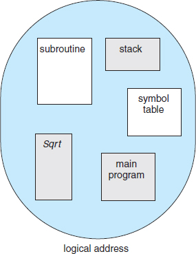
Figure 8.7 Programmer's view of a program.
For simplicity of implementation, segments are numbered and are referred to by a segment number, rather than by a segment name. Thus, a logical address consists of a two tuple:
<segment-number, offset>.
Normally, when a program is compiled, the compiler automatically constructs segments reflecting the input program.
A C compiler might create separate segments for the following:
- The code
- Global variables
- The heap, from which memory is allocated
- The stacks used by each thread
- The standard C library
Libraries that are linked in during compile time might be assigned separate segments. The loader would take all these segments and assign them segment numbers.
8.4.2 Segmentation Hardware
Although the programmer can now refer to objects in the program by a two-dimensional address, the actual physical memory is still, of course, a one-dimensional sequence of bytes. Thus, we must define an implementation to map two-dimensional user-defined addresses into one-dimensional physical addresses. This mapping is effected by a segment table. Each entry in the segment table has a segment base and a segment limit. The segment base contains the starting physical address where the segment resides in memory, and the segment limit specifies the length of the segment.
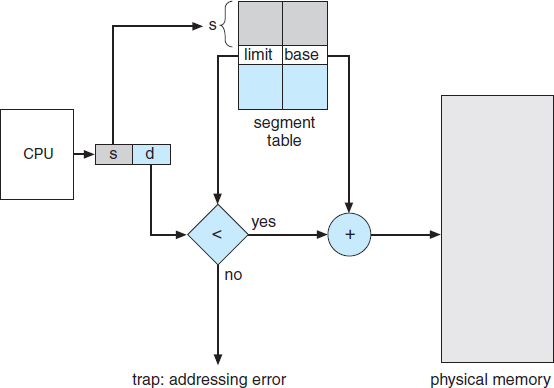
Figure 8.8 Segmentation hardware.
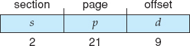
The use of a segment table is illustrated in Figure 8.8. A logical address consists of two parts: a segment number, s, and an offset into that segment, d. The segment number is used as an index to the segment table. The offset d of the logical address must be between 0 and the segment limit. If it is not, we trap to the operating system (logical addressing attempt beyond end of segment). When an offset is legal, it is added to the segment base to produce the address in physical memory of the desired byte. The segment table is thus essentially an array of base–limit register pairs.
As an example, consider the situation shown in Figure 8.9. We have five segments numbered from 0 through 4. The segments are stored in physical memory as shown. The segment table has a separate entry for each segment, giving the beginning address of the segment in physical memory (or base) and the length of that segment (or limit). For example, segment 2 is 400 bytes long and begins at location 4300. Thus, a reference to byte 53 of segment 2 is mapped onto location 4300 + 53 = 4353. A reference to segment 3, byte 852, is mapped to 3200 (the base of segment 3) + 852 = 4052. A reference to byte 1222 of segment 0 would result in a trap to the operating system, as this segment is only 1,000 bytes long.
8.5 Paging
Segmentation permits the physical address space of a process to be noncontiguous. Paging is another memory-management scheme that offers this advantage. However, paging avoids external fragmentation and the need for compaction, whereas segmentation does not. It also solves the considerable problem of fitting memory chunks of varying sizes onto the backing store. Most memory-management schemes used before the introduction of paging suffered from this problem. The problem arises because, when code fragments or data residing in main memory need to be swapped out, space must be found on the backing store. The backing store has the same fragmentation problems discussed in connection with main memory, but access is much slower, so compaction is impossible. Because of its advantages over earlier methods, paging in its various forms is used in most operating systems, from those for mainframes through those for smartphones. Paging is implemented through cooperation between the operating system and the computer hardware.
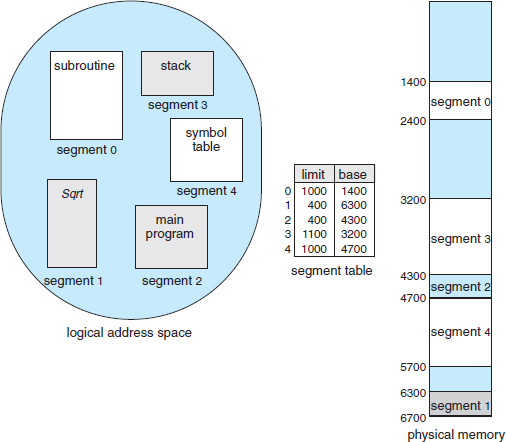
Figure 8.9 Example of segmentation.
8.5.1 Basic Method
The basic method for implementing paging involves breaking physical memory into fixed-sized blocks called frames and breaking logical memory into blocks of the same size called pages. When a process is to be executed, its pages are loaded into any available memory frames from their source (a file system or the backing store). The backing store is divided into fixed-sized blocks that are the same size as the memory frames or clusters of multiple frames. This rather simple idea has great functionality and wide ramifications. For example, the logical address space is now totally separate from the physical address space, so a process can have a logical 64-bit address space even though the system has less than 264 bytes of physical memory.
The hardware support for paging is illustrated in Figure 8.10. Every address generated by the CPU is divided into two parts: a page number (p) and a page offset (d). The page number is used as an index into a page table. The page table contains the base address of each page in physical memory. This base address is combined with the page offset to define the physical memory address that is sent to the memory unit. The paging model of memory is shown in Figure 8.11.
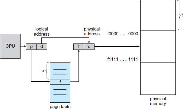
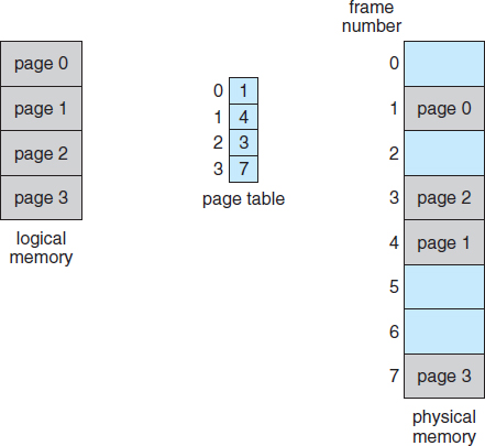
Figure 8.11 Paging model of logical and physical memory.
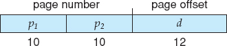
The page size (like the frame size) is defined by the hardware. The size of a page is a power of 2, varying between 512 bytes and 1 GB per page, depending on the computer architecture. The selection of a power of 2 as a page size makes the translation of a logical address into a page number and page offset particularly easy. If the size of the logical address space is 2m, and a page size is 2n bytes, then the high-order m − n bits of a logical address designate the page number, and the n low-order bits designate the page offset. Thus, the logical address is as follows:
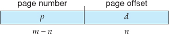
where p is an index into the page table and d is the displacement within the page.
As a concrete (although minuscule) example, consider the memory in Figure 8.12. Here, in the logical address, n = 2 and m = 4. Using a page size of 4 bytes and a physical memory of 32 bytes (8 pages), we show how the programmer's view of memory can be mapped into physical memory. Logical address 0 is page 0, offset 0. Indexing into the page table, we find that page 0 is in frame 5. Thus, logical address 0 maps to physical address 20 [= (5 × 4) + 0]. Logical address 3 (page 0, offset 3) maps to physical address 23 [= (5 × 4) + 3]. Logical address 4 is page 1, offset 0; according to the page table, page 1 is mapped to frame 6. Thus, logical address 4 maps to physical address 24 [= (6 × 4) + 0]. Logical address 13 maps to physical address 9.
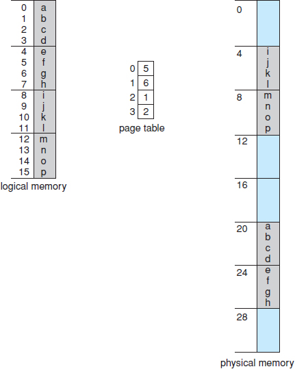
Figure 8.12 Paging example for a 32-byte memory with 4-byte pages.
OBTAINING THE PAGE SIZE ON LINUX SYSTEMS
On a Linux system, the page size varies according to architecture, and there are several ways of obtaining the page size. One approach is to use the getpagesize() system call. Another strategy is to enter the following command on the command line:
getconf PAGESIZE
Each of these techniques returns the page size as a number of bytes.
You may have noticed that paging itself is a form of dynamic relocation. Every logical address is bound by the paging hardware to some physical address. Using paging is similar to using a table of base (or relocation) registers, one for each frame of memory.
When we use a paging scheme, we have no external fragmentation: any free frame can be allocated to a process that needs it. However, we may have some internal fragmentation. Notice that frames are allocated as units. If the memory requirements of a process do not happen to coincide with page boundaries, the last frame allocated may not be completely full. For example, if page size is 2,048 bytes, a process of 72,766 bytes will need 35 pages plus 1,086 bytes. It will be allocated 36 frames, resulting in internal fragmentation of 2,048 − 1,086 = 962 bytes. In the worst case, a process would need n pages plus 1 byte. It would be allocated n + 1 frames, resulting in internal fragmentation of almost an entire frame.
If process size is independent of page size, we expect internal fragmentation to average one-half page per process. This consideration suggests that small page sizes are desirable. However, overhead is involved in each page-table entry, and this overhead is reduced as the size of the pages increases. Also, disk I/O is more efficient when the amount data being transferred is larger (Chapter 10). Generally, page sizes have grown over time as processes, data sets, and main memory have become larger. Today, pages typically are between 4 KB and 8 KB in size, and some systems support even larger page sizes. Some CPUs and kernels even support multiple page sizes. For instance, Solaris uses page sizes of 8 KB and 4 MB, depending on the data stored by the pages. Researchers are now developing support for variable on-the-fly page size.
Frequently, on a 32-bit CPU, each page-table entry is 4 bytes long, but that size can vary as well. A 32-bit entry can point to one of 232 physical page frames. If frame size is 4 KB (212), then a system with 4-byte entries can address 244 bytes (or 16 TB) of physical memory. We should note here that the size of physical memory in a paged memory system is different from the maximum logical size of a process. As we further explore paging, we introduce other information that must be kept in the page-table entries. That information reduces the number of bits available to address page frames. Thus, a system with 32-bit page-table entries may address less physical memory than the possible maximum. A 32-bit CPU uses 32-bit addresses, meaning that a given process space can only be 232 bytes (4 TB). Therefore, paging lets us use physical memory that is larger than what can be addressed by the CPU's address pointer length.
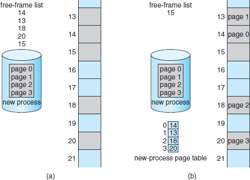
Figure 8.13 Free frames (a) before allocation and (b) after allocation.
When a process arrives in the system to be executed, its size, expressed in pages, is examined. Each page of the process needs one frame. Thus, if the process requires n pages, at least n frames must be available in memory. If n frames are available, they are allocated to this arriving process. The first page of the process is loaded into one of the allocated frames, and the frame number is put in the page table for this process. The next page is loaded into another frame, its frame number is put into the page table, and so on (Figure 8.13).
An important aspect of paging is the clear separation between the programmer's view of memory and the actual physical memory. The programmer views memory as one single space, containing only this one program. In fact, the user program is scattered throughout physical memory, which also holds other programs. The difference between the programmer's view of memory and the actual physical memory is reconciled by the address-translation hardware. The logical addresses are translated into physical addresses. This mapping is hidden from the programmer and is controlled by the operating system. Notice that the user process by definition is unable to access memory it does not own. It has no way of addressing memory outside of its page table, and the table includes only those pages that the process owns.
Since the operating system is managing physical memory, it must be aware of the allocation details of physical memory—which frames are allocated, which frames are available, how many total frames there are, and so on. This information is generally kept in a data structure called a frame table. The frame table has one entry for each physical page frame, indicating whether the latter is free or allocated and, if it is allocated, to which page of which process or processes.
In addition, the operating system must be aware that user processes operate in user space, and all logical addresses must be mapped to produce physical addresses. If a user makes a system call (to do I/O, for example) and provides an address as a parameter (a buffer, for instance), that address must be mapped to produce the correct physical address. The operating system maintains a copy of the page table for each process, just as it maintains a copy of the instruction counter and register contents. This copy is used to translate logical addresses to physical addresses whenever the operating system must map a logical address to a physical address manually. It is also used by the CPU dispatcher to define the hardware page table when a process is to be allocated the CPU. Paging therefore increases the context-switch time.
8.5.2 Hardware Support
Each operating system has its own methods for storing page tables. Some allocate a page table for each process. A pointer to the page table is stored with the other register values (like the instruction counter) in the process control block. When the dispatcher is told to start a process, it must reload the user registers and define the correct hardware page-table values from the stored user page table. Other operating systems provide one or at most a few page tables, which decreases the overhead involved when processes are context-switched.
The hardware implementation of the page table can be done in several ways. In the simplest case, the page table is implemented as a set of dedicated registers. These registers should be built with very high-speed logic to make the paging-address translation efficient. Every access to memory must go through the paging map, so efficiency is a major consideration. The CPU dispatcher reloads these registers, just as it reloads the other registers. Instructions to load or modify the page-table registers are, of course, privileged, so that only the operating system can change the memory map. The DEC PDP-11 is an example of such an architecture. The address consists of 16 bits, and the page size is 8 KB. The page table thus consists of eight entries that are kept in fast registers.
The use of registers for the page table is satisfactory if the page table is reasonably small (for example, 256 entries). Most contemporary computers, however, allow the page table to be very large (for example, 1 million entries). For these machines, the use of fast registers to implement the page table is not feasible. Rather, the page table is kept in main memory, and a page-table base register (PTBR) points to the page table. Changing page tables requires changing only this one register, substantially reducing context-switch time.
The problem with this approach is the time required to access a user memory location. If we want to access location i, we must first index into the page table, using the value in the PTBR offset by the page number for i. This task requires a memory access. It provides us with the frame number, which is combined with the page offset to produce the actual address. We can then access the desired place in memory. With this scheme, two memory accesses are needed to access a byte (one for the page-table entry, one for the byte). Thus, memory access is slowed by a factor of 2. This delay would be intolerable under most circumstances. We might as well resort to swapping!
The standard solution to this problem is to use a special, small, fast-lookup hardware cache called a translation look-aside buffer (TLB). The TLB is associative, high-speed memory. Each entry in the TLB consists of two parts: a key (or tag) and a value. When the associative memory is presented with an item, the item is compared with all keys simultaneously. If the item is found, the corresponding value field is returned. The search is fast; a TLB lookup in modern hardware is part of the instruction pipeline, essentially adding no performance penalty. To be able to execute the search within a pipeline step, however, the TLB must be kept small. It is typically between 32 and 1,024 entries in size. Some CPUs implement separate instruction and data address TLBs. That can double the number of TLB entries available, because those lookups occur in different pipeline steps. We can see in this development an example of the evolution of CPU technology: systems have evolved from having no TLBs to having multiple levels of TLBs, just as they have multiple levels of caches.
The TLB is used with page tables in the following way. The TLB contains only a few of the page-table entries. When a logical address is generated by the CPU, its page number is presented to the TLB. If the page number is found, its frame number is immediately available and is used to access memory. As just mentioned, these steps are executed as part of the instruction pipeline within the CPU, adding no performance penalty compared with a system that does not implement paging.
If the page number is not in the TLB (known as a TLB miss), a memory reference to the page table must be made. Depending on the CPU, this may be done automatically in hardware or via an interrupt to the operating system. When the frame number is obtained, we can use it to access memory (Figure 8.14). In addition, we add the page number and frame number to the TLB, so that they will be found quickly on the next reference. If the TLB is already full of entries, an existing entry must be selected for replacement. Replacement policies range from least recently used (LRU) through round-robin to random. Some CPUs allow the operating system to participate in LRU entry replacement, while others handle the matter themselves. Furthermore, some TLBs allow certain entries to be wired down, meaning that they cannot be removed from the TLB. Typically, TLB entries for key kernel code are wired down.
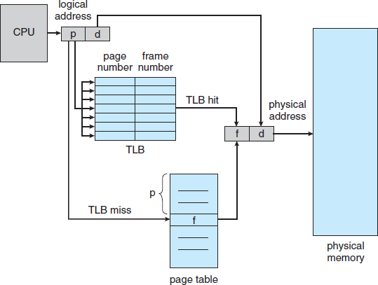
Figure 8.14 Paging hardware with TLB.
Some TLBs store address-space identifiers (ASIDs) in each TLB entry. An ASID uniquely identifies each process and is used to provide address-space protection for that process. When the TLB attempts to resolve virtual page numbers, it ensures that the ASID for the currently running process matches the ASID associated with the virtual page. If the ASIDs do not match, the attempt is treated as a TLB miss. In addition to providing address-space protection, an ASID allows the TLB to contain entries for several different processes simultaneously. If the TLB does not support separate ASIDs, then every time a new page table is selected (for instance, with each context switch), the TLB must be flushed (or erased) to ensure that the next executing process does not use the wrong translation information. Otherwise, the TLB could include old entries that contain valid virtual addresses but have incorrect or invalid physical addresses left over from the previous process.
The percentage of times that the page number of interest is found in the TLB is called the hit ratio. An 80-percent hit ratio, for example, means that we find the desired page number in the TLB 80 percent of the time. If it takes 100 nanoseconds to access memory, then a mapped-memory access takes 100 nanoseconds when the page number is in the TLB. If we fail to find the page number in the TLB then we must first access memory for the page table and frame number (100 nanoseconds) and then access the desired byte in memory (100 nanoseconds), for a total of 200 nanoseconds. (We are assuming that a page-table lookup takes only one memory access, but it can take more, as we shall see.) To find the effective memory-access time, we weight the case by its probability:
| effective access time | = 0.80 × 100 + 0.20 × 200 |
| = 120 nanoseconds |
In this example, we suffer a 20-percent slowdown in average memory-access time (from 100 to 120 nanoseconds).
For a 99-percent hit ratio, which is much more realistic, we have
| effective access time | = 0.99 × 100 + 0.01 × 200 |
| = 101 nanoseconds |
This increased hit rate produces only a 1 percent slowdown in access time.
As we noted earlier, CPUs today may provide multiple levels of TLBs. Calculating memory access times in modern CPUs is therefore much more complicated than shown in the example above. For instance, the Intel Core i7 CPU has a 128-entry L1 instruction TLB and a 64-entry L1 data TLB. In the case of a miss at L1, it takes the CPU six cycles to check for the entry in the L2 512-entry TLB. A miss in L2 means that the CPU must either walk through the page-table entries in memory to find the associated frame address, which can take hundreds of cycles, or interrupt to the operating system to have it do the work.
A complete performance analysis of paging overhead in such a system would require miss-rate information about each TLB tier. We can see from the general information above, however, that hardware features can have a significant effect on memory performance and that operating-system improvements (such as paging) can result in and, in turn, be affected by hardware changes (such as TLBs). We will further explore the impact of the hit ratio on the TLB in Chapter 9.
TLBs are a hardware feature and therefore would seem to be of little concern to operating systems and their designers. But the designer needs to understand the function and features of TLBs, which vary by hardware platform. For optimal operation, an operating-system design for a given platform must implement paging according to the platform's TLB design. Likewise, a change in the TLB design (for example, between generations of Intel CPUs) may necessitate a change in the paging implementation of the operating systems that use it.
8.5.3 Protection
Memory protection in a paged environment is accomplished by protection bits associated with each frame. Normally, these bits are kept in the page table.
One bit can define a page to be read–write or read-only. Every reference to memory goes through the page table to find the correct frame number. At the same time that the physical address is being computed, the protection bits can be checked to verify that no writes are being made to a read-only page. An attempt to write to a read-only page causes a hardware trap to the operating system (or memory-protection violation).
We can easily expand this approach to provide a finer level of protection. We can create hardware to provide read-only, read–write, or execute-only protection; or, by providing separate protection bits for each kind of access, we can allow any combination of these accesses. Illegal attempts will be trapped to the operating system.
One additional bit is generally attached to each entry in the page table: a valid–invalid bit. When this bit is set to valid, the associated page is in the process's logical address space and is thus a legal (or valid) page. When the bit is set toinvalid, the page is not in the process's logical address space. Illegal addresses are trapped by use of the valid–invalid bit. The operating system sets this bit for each page to allow or disallow access to the page.
Suppose, for example, that in a system with a 14-bit address space (0 to 16383), we have a program that should use only addresses 0 to 10468. Given a page size of 2 KB, we have the situation shown in Figure 8.15. Addresses in pages 0, 1, 2, 3, 4, and 5 are mapped normally through the page table. Any attempt to generate an address in pages 6 or 7, however, will find that the valid–invalid bit is set to invalid, and the computer will trap to the operating system (invalid page reference).
Notice that this scheme has created a problem. Because the program extends only to address 10468, any reference beyond that address is illegal. However, references to page 5 are classified as valid, so accesses to addresses up to 12287 are valid. Only the addresses from 12288 to 16383 are invalid. This problem is a result of the 2-KB page size and reflects the internal fragmentation of paging.
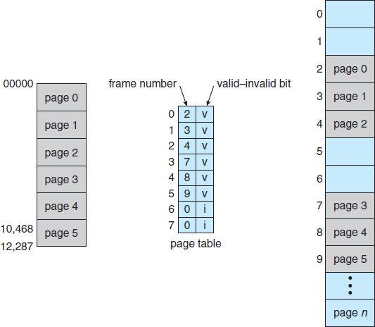
Figure 8.15 Valid (v) or invalid (i) bit in a page table.
Rarely does a process use all its address range. In fact, many processes use only a small fraction of the address space available to them. It would be wasteful in these cases to create a page table with entries for every page in the address range. Most of this table would be unused but would take up valuable memory space. Some systems provide hardware, in the form of a page-table length register (PTLR), to indicate the size of the page table. This value is checked against every logical address to verify that the address is in the valid range for the process. Failure of this test causes an error trap to the operating system.
8.5.4 Shared Pages
An advantage of paging is the possibility of sharing common code. This consideration is particularly important in a time-sharing environment. Consider a system that supports 40 users, each of whom executes a text editor. If the text editor consists of 150 KB of code and 50 KB of data space, we need 8,000 KB to support the 40 users. If the code is reentrant code (or pure code), however, it can be shared, as shown in Figure 8.16. Here, we see three processes sharing a three-page editor—each page 50 KB in size (the large page size is used to simplify the figure). Each process has its own data page.
Reentrant code is non-self-modifying code: it never changes during execution. Thus, two or more processes can execute the same code at the same time. Each process has its own copy of registers and data storage to hold the data for the process's execution. The data for two different processes will, of course, be different.
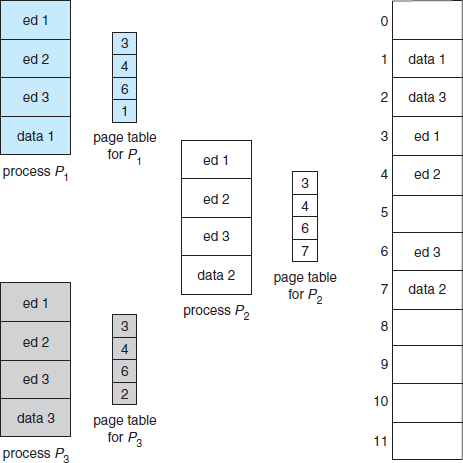
Figure 8.16 Sharing of code in a paging environment.
Only one copy of the editor need be kept in physical memory. Each user's page table maps onto the same physical copy of the editor, but data pages are mapped onto different frames. Thus, to support 40 users, we need only one copy of the editor (150 KB), plus 40 copies of the 50 KB of data space per user. The total space required is now 2,150 KB instead of 8,000 KB—a significant savings.
Other heavily used programs can also be shared—compilers, window systems, run-time libraries, database systems, and so on. To be sharable, the code must be reentrant. The read-only nature of shared code should not be left to the correctness of the code; the operating system should enforce this property.
The sharing of memory among processes on a system is similar to the sharing of the address space of a task by threads, described in Chapter 4. Furthermore, recall that in Chapter 3 we described shared memory as a method of interprocess communication. Some operating systems implement shared memory using shared pages.
Organizing memory according to pages provides numerous benefits in addition to allowing several processes to share the same physical pages. We cover several other benefits in Chapter 9.
8.6 Structure of the Page Table
In this section, we explore some of the most common techniques for structuring the page table, including hierarchical paging, hashed page tables, and inverted page tables.
8.6.1 Hierarchical Paging
Most modern computer systems support a large logical address space (232 to 264). In such an environment, the page table itself becomes excessively large. For example, consider a system with a 32-bit logical address space. If the page size in such a system is 4 KB (212), then a page table may consist of up to 1 million entries (232/212). Assuming that each entry consists of 4 bytes, each process may need up to 4 MB of physical address space for the page table alone. Clearly, we would not want to allocate the page table contiguously in main memory. One simple solution to this problem is to divide the page table into smaller pieces. We can accomplish this division in several ways.
One way is to use a two-level paging algorithm, in which the page table itself is also paged (Figure 8.17). For example, consider again the system with a 32-bit logical address space and a page size of 4 KB. A logical address is divided into a page number consisting of 20 bits and a page offset consisting of 12 bits. Because we page the page table, the page number is further divided into a 10-bit page number and a 10-bit page offset. Thus, a logical address is as follows:
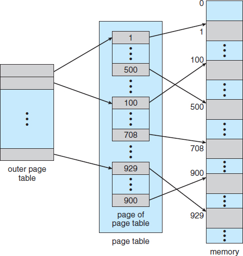
Figure 8.17 A two-level page-table scheme.
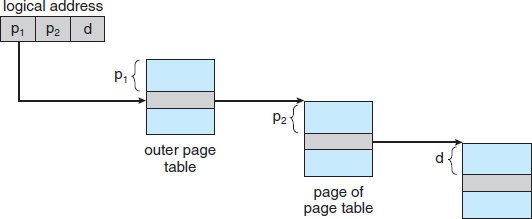
Figure 8.18 Address translation for a two-level 32-bit paging architecture.
where p1 is an index into the outer page table and p2 is the displacement within the page of the inner page table. The address-translation method for this architecture is shown in Figure 8.18. Because address translation works from the outer page table inward, this scheme is also known as a forward-mapped page table.
Consider the memory management of one of the classic systems, the VAX minicomputer from Digital Equipment Corporation (DEC). The VAX was the most popular minicomputer of its time and was sold from 1977 through 2000. The VAX architecture supported a variation of two-level paging. The VAX is a 32-bit machine with a page size of 512 bytes. The logical address space of a process is divided into four equal sections, each of which consists of 230 bytes. Each section represents a different part of the logical address space of a process. The first 2 high-order bits of the logical address designate the appropriate section. The next 21 bits represent the logical page number of that section, and the final 9 bits represent an offset in the desired page. By partitioning the page table in this manner, the operating system can leave partitions unused until a process needs them. Entire sections of virtual address space are frequently unused, and multilevel page tables have no entries for these spaces, greatly decreasing the amount of memory needed to store virtual memory data structures.
An address on the VAX architecture is as follows:
where s designates the section number, p is an index into the page table, and d is the displacement within the page. Even when this scheme is used, the size of a one-level page table for a VAX process using one section is 221 bits * 4 bytes per entry = 8 MB. To further reduce main-memory use, the VAX pages the user-process page tables.
For a system with a 64-bit logical address space, a two-level paging scheme is no longer appropriate. To illustrate this point, let's suppose that the page size in such a system is 4 KB (212). In this case, the page table consists of up to 252 entries. If we use a two-level paging scheme, then the inner page tables can conveniently be one page long, or contain 210 4-byte entries. The addresses look like this:
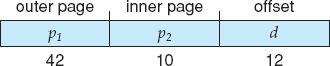
The outer page table consists of 242 entries, or 244 bytes. The obvious way to avoid such a large table is to divide the outer page table into smaller pieces. (This approach is also used on some 32-bit processors for added flexibility and efficiency.)
We can divide the outer page table in various ways. For example, we can page the outer page table, giving us a three-level paging scheme. Suppose that the outer page table is made up of standard-size pages (210 entries, or 212 bytes). In this case, a 64-bit address space is still daunting:
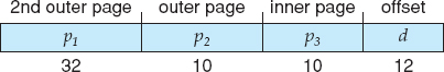
The outer page table is still 234 bytes (16 GB) in size.
The next step would be a four-level paging scheme, where the second-level outer page table itself is also paged, and so forth. The 64-bit UltraSPARC would require seven levels of paging—a prohibitive number of memory accesses—to translate each logical address. You can see from this example why, for 64-bit architectures, hierarchical page tables are generally considered inappropriate.
8.6.2 Hashed Page Tables
A common approach for handling address spaces larger than 32 bits is to use a hashed page table, with the hash value being the virtual page number. Each entry in the hash table contains a linked list of elements that hash to the same location (to handle collisions). Each element consists of three fields: (1) the virtual page number, (2) the value of the mapped page frame, and (3) a pointer to the next element in the linked list.
The algorithm works as follows: The virtual page number in the virtual address is hashed into the hash table. The virtual page number is compared with field 1 in the first element in the linked list. If there is a match, the corresponding page frame (field 2) is used to form the desired physical address. If there is no match, subsequent entries in the linked list are searched for a matching virtual page number. This scheme is shown in Figure 8.19.
A variation of this scheme that is useful for 64-bit address spaces has been proposed. This variation uses clustered page tables, which are similar to hashed page tables except that each entry in the hash table refers to several pages (such as 16) rather than a single page. Therefore, a single page-table entry can store the mappings for multiple physical-page frames. Clustered page tables are particularly useful for sparse address spaces, where memory references are noncontiguous and scattered throughout the address space.
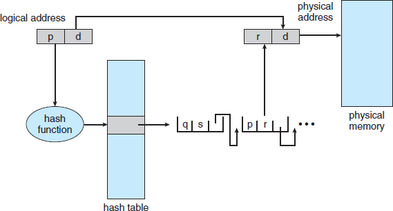
Figure 8.19 Hashed page table.
8.6.3 Inverted Page Tables
Usually, each process has an associated page table. The page table has one entry for each page that the process is using (or one slot for each virtual address, regardless of the latter's validity). This table representation is a natural one, since processes reference pages through the pages' virtual addresses. The operating system must then translate this reference into a physical memory address. Since the table is sorted by virtual address, the operating system is able to calculate where in the table the associated physical address entry is located and to use that value directly. One of the drawbacks of this method is that each page table may consist of millions of entries. These tables may consume large amounts of physical memory just to keep track of how other physical memory is being used.
To solve this problem, we can use an inverted page table. An inverted page table has one entry for each real page (or frame) of memory. Each entry consists of the virtual address of the page stored in that real memory location, with information about the process that owns the page. Thus, only one page table is in the system, and it has only one entry for each page of physical memory. Figure 8.20 shows the operation of an inverted page table. Compare it with Figure 8.10, which depicts a standard page table in operation. Inverted page tables often require that an address-space identifier (Section 8.5.2) be stored in each entry of the page table, since the table usually contains several different address spaces mapping physical memory. Storing the address-space identifier ensures that a logical page for a particular process is mapped to the corresponding physical page frame. Examples of systems using inverted page tables include the 64-bit UltraSPARC and PowerPC.
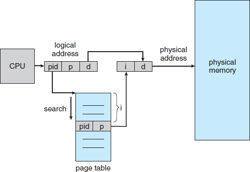
Figure 8.20 Inverted page table.
To illustrate this method, we describe a simplified version of the inverted page table used in the IBM RT. IBM was the first major company to use inverted page tables, starting with the IBM System 38 and continuing through the RS/6000 and the current IBM Power CPUs. For the IBM RT, each virtual address in the system consists of a triple:
<process-id, page-number, offset>.
Each inverted page-table entry is a pair <process-id, page-number> where the process-id assumes the role of the address-space identifier. When a memory reference occurs, part of the virtual address, consisting of <process-id, page-number>, is presented to the memory subsystem. The inverted page table is then searched for a match. If a match is found—say, at entry i—then the physical address <i, offset> is generated. If no match is found, then an illegal address access has been attempted.
Although this scheme decreases the amount of memory needed to store each page table, it increases the amount of time needed to search the table when a page reference occurs. Because the inverted page table is sorted by physical address, but lookups occur on virtual addresses, the whole table might need to be searched before a match is found. This search would take far too long. To alleviate this problem, we use a hash table, as described in Section 8.6.2, to limit the search to one—or at most a few—page-table entries. Of course, each access to the hash table adds a memory reference to the procedure, so one virtual memory reference requires at least two real memory reads—one for the hash-table entry and one for the page table. (Recall that the TLB is searched first, before the hash table is consulted, offering some performance improvement.)
Systems that use inverted page tables have difficulty implementing shared memory. Shared memory is usually implemented as multiple virtual addresses (one for each process sharing the memory) that are mapped to one physical address. This standard method cannot be used with inverted page tables; because there is only one virtual page entry for every physical page, one physical page cannot have two (or more) shared virtual addresses. A simple technique for addressing this issue is to allow the page table to contain only one mapping of a virtual address to the shared physical address. This means that references to virtual addresses that are not mapped result in page faults.
8.6.4 Oracle SPARC Solaris
Consider as a final example a modern 64-bit CPU and operating system that are tightly integrated to provide low-overhead virtual memory. Solaris running on the SPARC CPU is a fully 64-bit operating system and as such has to solve the problem of virtual memory without using up all of its physical memory by keeping multiple levels of page tables. Its approach is a bit complex but solves the problem efficiently using hashed page tables. There are two hash tables—one for the kernel and one for all user processes. Each maps memory addresses from virtual to physical memory. Each hash-table entry represents a contiguous area of mapped virtual memory, which is more efficient than having a separate hash-table entry for each page. Each entry has a base address and a span indicating the number of pages the entry represents.
Virtual-to-physical translation would take too long if each address required searching through a hash table, so the CPU implements a TLB that holds translation table entries (TTEs) for fast hardware lookups. A cache of these TTEs reside in a translation storage buffer (TSB), which includes an entry per recently accessed page. When a virtual address reference occurs, the hardware searches the TLB for a translation. If none is found, the hardware walks through the in-memory TSB looking for the TTE that corresponds to the virtual address that caused the lookup. This TLB walk functionality is found on many modern CPUs. If a match is found in the TSB, the CPU copies the TSB entry into the TLB, and the memory translation completes. If no match is found in the TSB, the kernel is interrupted to search the hash table. The kernel then creates a TTE from the appropriate hash table and stores it in the TSB for automatic loading into the TLB by the CPU memory-management unit. Finally, the interrupt handler returns control to the MMU, which completes the address translation and retrieves the requested byte or word from main memory.
8.7 Example: Intel 32 and 64-bit Architectures
The architecture of Intel chips has dominated the personal computer landscape for several years. The 16-bit Intel 8086 appeared in the late 1970s and was soon followed by another 16-bit chip—the Intel 8088—which was notable for being the chip used in the original IBM PC. Both the 8086 chip and the 8088 chip were based on a segmented architecture. Intel later produced a series of 32-bit chips—the IA-32—which included the family of 32-bit Pentium processors. The IA-32 architecture supported both paging and segmentation. More recently, Intel has produced a series of 64-bit chips based on the x86-64 architecture. Currently, all the most popular PC operating systems run on Intel chips, including Windows, Mac OS X, and Linux (although Linux, of course, runs on several other architectures as well). Notably, however, Intel's dominance has not spread to mobile systems, where the ARM architecture currently enjoys considerable success (see Section 8.8).
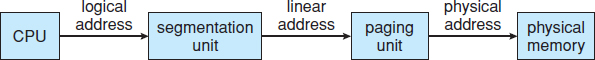
Figure 8.21 Logical to physical address translation in IA-32.
In this section, we examine address translation for both IA-32 and x86-64 architectures. Before we proceed, however, it is important to note that because Intel has released several versions—as well as variations—of its architectures over the years, we cannot provide a complete description of the memory-management structure of all its chips. Nor can we provide all of the CPU details, as that information is best left to books on computer architecture. Rather, we present the major memory-management concepts of these Intel CPUs.
8.7.1 IA-32 Architecture
Memory management in IA-32 systems is divided into two components—segmentation and paging—and works as follows: The CPU generates logical addresses, which are given to the segmentation unit. The segmentation unit produces a linear address for each logical address. The linear address is then given to the paging unit, which in turn generates the physical address in main memory. Thus, the segmentation and paging units form the equivalent of the memory-management unit (MMU). This scheme is shown in Figure 8.21.
8.7.1.1 IA-32 Segmentation
The IA-32 architecture allows a segment to be as large as 4 GB, and the maximum number of segments per process is 16 K. The logical address space of a process is divided into two partitions. The first partition consists of up to 8 K segments that are private to that process. The second partition consists of up to 8 K segments that are shared among all the processes. Information about the first partition is kept in the local descriptor table (LDT); information about the second partition is kept in the global descriptor table (GDT). Each entry in the LDT and GDT consists of an 8-byte segment descriptor with detailed information about a particular segment, including the base location and limit of that segment.
The logical address is a pair (selector, offset), where the selector is a 16-bit number:
![]()
in which s designates the segment number, g indicates whether the segment is in the GDT or LDT, and p deals with protection. The offset is a 32-bit number specifying the location of the byte within the segment in question.
The machine has six segment registers, allowing six segments to be addressed at any one time by a process. It also has six 8-byte microprogram registers to hold the corresponding descriptors from either the LDT or GDT. This cache lets the Pentium avoid having to read the descriptor from memory for every memory reference.
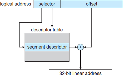
Figure 8.22 IA-32 segmentation.
The linear address on the IA-32 is 32 bits long and is formed as follows. The segment register points to the appropriate entry in the LDT or GDT. The base and limit information about the segment in question is used to generate a linear address. First, the limit is used to check for address validity. If the address is not valid, a memory fault is generated, resulting in a trap to the operating system. If it is valid, then the value of the offset is added to the value of the base, resulting in a 32-bit linear address. This is shown in Figure 8.22. In the following section, we discuss how the paging unit turns this linear address into a physical address.
8.7.1.2 IA-32 Paging
The IA-32 architecture allows a page size of either 4 KB or 4 MB. For 4-KB pages, IA-32 uses a two-level paging scheme in which the division of the 32-bit linear address is as follows:
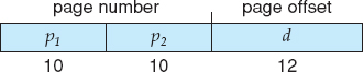
The address-translation scheme for this architecture is similar to the scheme shown in Figure 8.18. The IA-32 address translation is shown in more detail in Figure 8.23. The 10 high-order bits reference an entry in the outermost page table, which IA-32 terms the page directory. (The CR3 register points to the page directory for the current process.) The page directory entry points to an inner page table that is indexed by the contents of the innermost 10 bits in the linear address. Finally, the low-order bits 0–11 refer to the offset in the 4-KB page pointed to in the page table.
One entry in the page directory is the Page_Size flag, which—if set—indicates that the size of the page frame is 4 MB and not the standard 4 KB. If this flag is set, the page directory points directly to the 4-MB page frame, bypassing the inner page table; and the 22 low-order bits in the linear address refer to the offset in the 4-MB page frame.
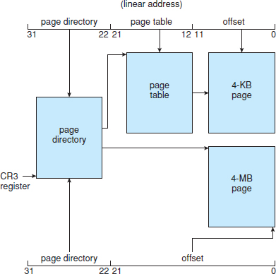
Figure 8.23 Paging in the IA-32 architecture.
To improve the efficiency of physical memory use, IA-32 page tables can be swapped to disk. In this case, an invalid bit is used in the page directory entry to indicate whether the table to which the entry is pointing is in memory or on disk. If the table is on disk, the operating system can use the other 31 bits to specify the disk location of the table. The table can then be brought into memory on demand.
As software developers began to discover the 4-GB memory limitations of 32-bit architectures, Intel adopted a page address extension (PAE), which allows 32-bit processors to access a physical address space larger than 4 GB. The fundamental difference introduced by PAE support was that paging went from a two-level scheme (as shown in Figure 8.23) to a three-level scheme, where the top two bits refer to a page directory pointer table. Figure 8.24 illustrates a PAE system with 4-KB pages. (PAE also supports 2-MB pages.)
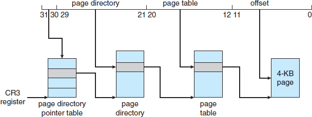
Figure 8.24 Page address extensions.

Figure 8.25 x86-64 linear address.
PAE also increased the page-directory and page-table entries from 32 to 64 bits in size, which allowed the base address of page tables and page frames to extend from 20 to 24 bits. Combined with the 12-bit offset, adding PAE support to IA-32 increased the address space to 36 bits, which supports up to 64 GB of physical memory. It is important to note that operating system support is required to use PAE. Both Linux and Intel Mac OS X support PAE. However, 32-bit versions of Windows desktop operating systems still provide support for only 4 GB of physical memory, even if PAE is enabled.
8.7.2 x86-64
Intel has had an interesting history of developing 64-bit architectures. Its initial entry was the IA-64 (later named Itanium) architecture, but that architecture was not widely adopted. Meanwhile, another chip manufacturer—AMD —began developing a 64-bit architecture known as x86-64 that was based on extending the existing IA-32 instruction set. The x86-64 supported much larger logical and physical address spaces, as well as several other architectural advances. Historically, AMD had often developed chips based on Intel's architecture, but now the roles were reversed as Intel adopted AMD's x86-64 architecture. In discussing this architecture, rather than using the commercial names AMD64 and Intel 64, we will use the more general term x86-64.
Support for a 64-bit address space yields an astonishing 264 bytes of addressable memory—a number greater than 16 quintillion (or 16 exabytes). However, even though 64-bit systems can potentially address this much memory, in practice far fewer than 64 bits are used for address representation in current designs. The x86-64 architecture currently provides a 48-bit virtual address with support for page sizes of 4 KB, 2 MB, or 1 GB using four levels of paging hierarchy. The representation of the linear address appears in Figure 8.25. Because this addressing scheme can use PAE, virtual addresses are 48 bits in size but support 52-bit physical addresses (4096 terabytes).
64-BIT COMPUTING
History has taught us that even though memory capacities, CPU speeds, and similar computer capabilities seem large enough to satisfy demand for the foreseeable future, the growth of technology ultimately absorbs available capacities, and we find ourselves in need of additional memory or processing power, often sooner than we think. What might the future of technology bring that would make a 64-bit address space seem too small?
8.8 Example: ARM Architecture
Although Intel chips have dominated the personal computer market for over 30 years, chips for mobile devices such as smartphones and tablet computers often instead run on 32-bit ARM processors. Interestingly, whereas Intel both designs and manufactures chips, ARM only designs them. It then licenses its designs to chip manufacturers. Apple has licensed the ARM design for its iPhone and iPad mobile devices, and several Android-based smartphones use ARM processors as well.
The 32-bit ARM architecture supports the following page sizes:
- 4-KB and 16-KB pages
- 1-MB and 16-MB pages (termed sections)
The paging system in use depends on whether a page or a section is being referenced. One-level paging is used for 1-MB and 16-MB sections; two-level paging is used for 4-KB and 16-KB pages. Address translation with the ARM MMU is shown in Figure 8.26.
The ARM architecture also supports two levels of TLBs. At the outer level are two micro TLBs—a separate TLB for data and another for instructions. The micro TLB supports ASIDs as well. At the inner level is a single main TLB. Address translation begins at the micro TLB level. In the case of a miss, the main TLB is then checked. If both TLBs yield misses, a page table walk must be performed in hardware.
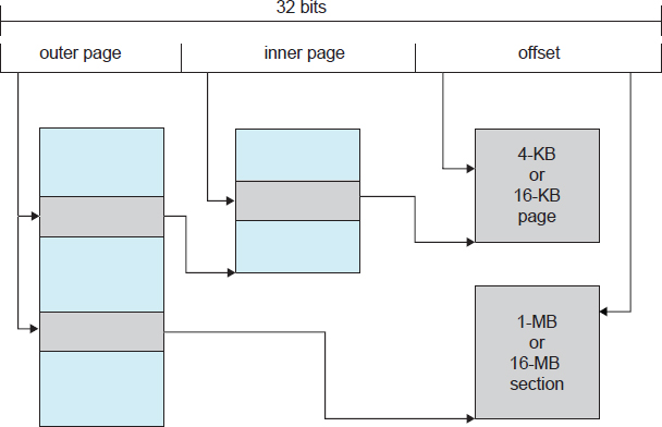
Figure 8.26 Logical address translation in ARM.
8.9 Summary
Memory-management algorithms for multiprogrammed operating systems range from the simple single-user system approach to segmentation and paging. The most important determinant of the method used in a particular system is the hardware provided. Every memory address generated by the CPU must be checked for legality and possibly mapped to a physical address. The checking cannot be implemented (efficiently) in software. Hence, we are constrained by the hardware available.
The various memory-management algorithms (contiguous allocation, paging, segmentation, and combinations of paging and segmentation) differ in many aspects. In comparing different memory-management strategies, we use the following considerations:
- Hardware support. A simple base register or a base–limit register pair is sufficient for the single- and multiple-partition schemes, whereas paging and segmentation need mapping tables to define the address map.
- Performance. As the memory-management algorithm becomes more complex, the time required to map a logical address to a physical address increases. For the simple systems, we need only compare or add to the logical address—operations that are fast. Paging and segmentation can be as fast if the mapping table is implemented in fast registers. If the table is in memory, however, user memory accesses can be degraded substantially. A TLB can reduce the performance degradation to an acceptable level.
- Fragmentation. A multiprogrammed system will generally perform more efficiently if it has a higher level of multiprogramming. For a given set of processes, we can increase the multiprogramming level only by packing more processes into memory. To accomplish this task, we must reduce memory waste, or fragmentation. Systems with fixed-sized allocation units, such as the single-partition scheme and paging, suffer from internal fragmentation. Systems with variable-sized allocation units, such as the multiple-partition scheme and segmentation, suffer from external fragmentation.
- Relocation. One solution to the external-fragmentation problem is compaction. Compaction involves shifting a program in memory in such a way that the program does not notice the change. This consideration requires that logical addresses be relocated dynamically, at execution time. If addresses are relocated only at load time, we cannot compact storage.
- Swapping. Swapping can be added to any algorithm. At intervals determined by the operating system, usually dictated by CPU-scheduling policies, processes are copied from main memory to a backing store and later are copied back to main memory. This scheme allows more processes to be run than can be fit into memory at one time. In general, PC operating systems support paging, and operating systems for mobile devices do not.
- Sharing. Another means of increasing the multiprogramming level is to share code and data among different processes. Sharing generally requires that either paging or segmentation be used to provide small packets of information (pages or segments) that can be shared. Sharing is a means of running many processes with a limited amount of memory, but shared programs and data must be designed carefully.
- Protection. If paging or segmentation is provided, different sections of a user program can be declared execute-only, read-only, or read–write. This restriction is necessary with shared code or data and is generally useful in any case to provide simple run-time checks for common programming errors.
Practice Exercises
8.1 Name two differences between logical and physical addresses.
8.2 Consider a system in which a program can be separated into two parts: code and data. The CPU knows whether it wants an instruction (instruction fetch) or data (data fetch or store). Therefore, two base–limit register pairs are provided: one for instructions and one for data. The instruction base–limit register pair is automatically read-only, so programs can be shared among different users. Discuss the advantages and disadvantages of this scheme.
8.3 Why are page sizes always powers of 2?
8.4 Consider a logical address space of 64 pages of 1,024 words each, mapped onto a physical memory of 32 frames.
- How many bits are there in the logical address?
- How many bits are there in the physical address?
8.5 What is the effect of allowing two entries in a page table to point to the same page frame in memory? Explain how this effect could be used to decrease the amount of time needed to copy a large amount of memory from one place to another. What effect would updating some byte on the one page have on the other page?
8.6 Describe a mechanism by which one segment could belong to the address space of two different processes.
8.7 Sharing segments among processes without requiring that they have the same segment number is possible in a dynamically linked segmentation system.
- Define a system that allows static linking and sharing of segments without requiring that the segment numbers be the same.
- Describe a paging scheme that allows pages to be shared without requiring that the page numbers be the same.
8.8 In the IBM/370, memory protection is provided through the use of keys. A key is a 4-bit quantity. Each 2-K block of memory has a key (the storage key) associated with it. The CPU also has a key (the protection key) associated with it. A store operation is allowed only if both keys are equal or if either is 0. Which of the following memory-management schemes could be used successfully with this hardware?
- Bare machine
- Single-user system
- Multiprogramming with a fixed number of processes
- Multiprogramming with a variable number of processes
- Paging
- Segmentation
Exercises
8.9 Explain the difference between internal and external fragmentation.
8.10 Consider the following process for generating binaries. A compiler is used to generate the object code for individual modules, and a linkage editor is used to combine multiple object modules into a single program binary. How does the linkage editor change the binding of instructions and data to memory addresses? What information needs to be passed from the compiler to the linkage editor to facilitate the memory-binding tasks of the linkage editor?
8.11 Given six memory partitions of 300 KB, 600 KB, 350 KB, 200 KB, 750 KB, and 125 KB (in order), how would the first-fit, best-fit, and worst-fit algorithms place processes of size 115 KB, 500 KB, 358 KB, 200 KB, and 375 KB (in order)? Rank the algorithms in terms of how efficiently they use memory.
8.12 Most systems allow a program to allocate more memory to its address space during execution. Allocation of data in the heap segments of programs is an example of such allocated memory. What is required to support dynamic memory allocation in the following schemes?
- Contiguous memory allocation
- Pure segmentation
- Pure paging
8.13 Compare the memory organization schemes of contiguous memory allocation, pure segmentation, and pure paging with respect to the following issues:
- External fragmentation
- Internal fragmentation
- Ability to share code across processes
8.14 On a system with paging, a process cannot access memory that it does not own. Why? How could the operating system allow access to other memory? Why should it or should it not?
8.15 Explain why mobile operating systems such as iOS and Android do not support swapping.
8.16 Although Android does not support swapping on its boot disk, it is possible to set up a swap space using a separate SD nonvolatile memory card. Why would Android disallow swapping on its boot disk yet allow it on a secondary disk?
8.17 Compare paging with segmentation with respect to how much memory the address translation structures require to convert virtual addresses to physical addresses.
8.18 Explain why address space identifiers (ASIDs) are used.
8.19 Program binaries in many systems are typically structured as follows. Code is stored starting with a small, fixed virtual address, such as 0. The code segment is followed by the data segment that is used for storing the program variables. When the program starts executing, the stack is allocated at the other end of the virtual address space and is allowed to grow toward lower virtual addresses. What is the significance of this structure for the following schemes?
- Contiguous memory allocation
- Pure segmentation
- Pure paging
8.20 Assuming a 1-KB page size, what are the page numbers and offsets for the following address references (provided as decimal numbers):
- 3085
- 42095
- 215201
- 650000
- 2000001
8.21 The BTV operating system has a 21-bit virtual address, yet on certain embedded devices, it has only a 16-bit physical address. It also has a 2-KB page size. How many entries are there in each of the following?
- A conventional, single-level page table
- An inverted page table
8.22 What is the maximum amount of physical memory?
8.23 Consider a logical address space of 256 pages with a 4-KB page size, mapped onto a physical memory of 64 frames.
- How many bits are required in the logical address?
- How many bits are required in the physical address?
8.24 Consider a computer system with a 32-bit logical address and 4-KB page size. The system supports up to 512 MB of physical memory. How many entries are there in each of the following?
8.25 Consider a paging system with the page table stored in memory.
- If a memory reference takes 50 nanoseconds, how long does a paged memory reference take?
- If we add TLBs, and 75 percent of all page-table references are found in the TLBs, what is the effective memory reference time? (Assume that finding a page-table entry in the TLBs takes 2 nanoseconds, if the entry is present.)
8.26 Why are segmentation and paging sometimes combined into one scheme?
8.27 Explain why sharing a reentrant module is easier when segmentation is used than when pure paging is used.
8.28 Consider the following segment table:
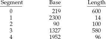
What are the physical addresses for the following logical addresses?
- 0,430
- 1,10
- 2,500
- 3,400
- 4,112
8.29 What is the purpose of paging the page tables?
8.30 Consider the hierarchical paging scheme used by the VAX architecture. How many memory operations are performed when a user program executes a memory-load operation?
8.31 Compare the segmented paging scheme with the hashed page table scheme for handling large address spaces. Under what circumstances is one scheme preferable to the other?
8.32 Consider the Intel address-translation scheme shown in Figure 8.22.
- Describe all the steps taken by the Intel Pentium in translating a logical address into a physical address.
- What are the advantages to the operating system of hardware that provides such complicated memory translation?
- Are there any disadvantages to this address-translation system? If so, what are they? If not, why is this scheme not used by every manufacturer?
Programming Problems
8.33 Assume that a system has a 32-bit virtual address with a 4-KB page size. Write a C program that is passed a virtual address (in decimal) on the command line and have it output the page number and offset for the given address. As an example, your program would run as follows:
./a.out 19986
Your program would output:
The address 19986 contains:
page number = 4
offset = 3602
Writing this program will require using the appropriate data type to store 32 bits. We encourage you to use unsigned data types as well.
Bibliographical Notes
Dynamic storage allocation was discussed by [Knuth (1973)] (Section 2.5), who found through simulation that first fit is generally superior to best fit. [Knuth (1973)] also discussed the 50-percent rule.
The concept of paging can be credited to the designers of the Atlas system, which has been described by [Kilburn et al. (1961)] and by [Howarth et al. (1961)]. The concept of segmentation was first discussed by [Dennis (1965)]. Paged segmentation was first supported in the GE 645, on which MULTICS was originally implemented ([Organick (1972)] and [Daley and Dennis (1967)]).
Inverted page tables are discussed in an article about the IBM RT storage manager by [Chang and Mergen (1988)].
[Hennessy and Patterson (2012)] explains the hardware aspects of TLBs, caches, and MMUs. [Talluri et al. (1995)] discusses page tables for 64-bit address spaces. [Jacob and Mudge (2001)] describes techniques for managing the TLB. [Fang et al. (2001)] evaluates support for large pages.
http://msdn.microsoft.com/en-us/library/windows/hardware/gg487512.aspx discusses PAE support for Windows systems.
http://www.intel.com/content/www/us/en/processors/architectures-software-developer-manuals.html provides various manuals for Intel 64 and IA-32 architectures.
http://www.arm.com/products/processors/cortex-a/cortex-a9.php provides an overview of the ARM architecture.
Bibliography
[Chang and Mergen (1988)] A. Chang and M. F. Mergen, “801 Storage: Architecture and Programming”, ACM Transactions on Computer Systems, Volume 6, Number 1 (1988), pages 28–50.
[Daley and Dennis (1967)] R. C. Daley and J. B. Dennis, “Virtual Memory, Processes, and Sharing in Multics”, Proceedings of the ACM Symposium on Operating Systems Principles (1967), pages 121–128.
[Dennis (1965)] J. B. Dennis, “Segmentation and the Design of Multiprogrammed Computer Systems”, Communications of the ACM, Volume 8, Number 4 (1965), pages 589–602.
[Fang et al. (2001)] Z. Fang, L.Zhang, J. B. Carter, W. C. Hsieh, and S. A. McKee, “Reevaluating Online Superpage Promotion with Hardware Support”, Proceedings of the International Symposium on High-Performance Computer Architecture, Volume 50, Number 5 (2001).
[Hennessy and Patterson (2012)] J. Hennessy and D. Patterson, Computer Architecture: A Quantitative Approach, Fifth Edition, Morgan Kaufmann (2012).
[Howarth et al. (1961)] D. J. Howarth, R. B. Payne, and F. H. Sumner, “The Manchester University Atlas Operating System, Part II: User's Description”, Computer Journal, Volume 4, Number 3 (1961), pages 226–229.
[Jacob and Mudge (2001)] B. Jacob and T. Mudge, “Uniprocessor Virtual Memory Without TLBs”, IEEE Transactions on Computers, Volume 50, Number 5 (2001).
[Kilburn et al. (1961)] T. Kilburn, D. J. Howarth, R. B. Payne, and F. H. Sumner, “The Manchester University Atlas Operating System, Part I: Internal Organization”, Computer Journal, Volume 4, Number 3 (1961), pages 222–225.
[Knuth (1973)] D. E. Knuth, The Art of Computer Programming, Volume 1: Fundamental Algorithms, Second Edition, Addison-Wesley (1973).
[Organick (1972)] E. I. Organick, The Multics System: An Examination of Its Structure, MIT Press (1972).
[Talluri et al. (1995)] M. Talluri, M. D. Hill, and Y. A. Khalidi, “A New Page Table for 64-bit Address Spaces”, Proceedings of the ACM Symposium on Operating Systems Principles (1995), pages 184–200.