CHAPTER 10

Mass-Storage Structure

The file system can be viewed logically as consisting of three parts. In Chapter 11, we examine the user and programmer interface to the file system. In Chapter 12, we describe the internal data structures and algorithms used by the operating system to implement this interface. In this chapter, we begin a discussion of file systems at the lowest level: the structure of secondary storage. We first describe the physical structure of magnetic disks and magnetic tapes. We then describe disk-scheduling algorithms, which schedule the order of disk I/Os to maximize performance. Next, we discuss disk formatting and management of boot blocks, damaged blocks, and swap space. We conclude with an examination of the structure of RAID systems.

10.1 Overview of Mass-Storage Structure

In this section, we present a general overview of the physical structure of secondary and tertiary storage devices.

10.1.1 Magnetic Disks

Magnetic disks provide the bulk of secondary storage for modern computer systems. Conceptually, disks are relatively simple (Figure 10.1). Each disk platter has a flat circular shape, like a CD. Common platter diameters range from 1.8 to 3.5 inches. The two surfaces of a platter are covered with a magnetic material. We store information by recording it magnetically on the platters.

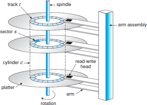
Figure 10.1 Moving-head disk mechanism.

A read–write head “flies” just above each surface of every platter. The heads are attached to a disk arm that moves all the heads as a unit. The surface of a platter is logically divided into circular tracks, which are subdivided into sectors. The set of tracks that are at one arm position makes up a cylinder. There may be thousands of concentric cylinders in a disk drive, and each track may contain hundreds of sectors. The storage capacity of common disk drives is measured in gigabytes.

When the disk is in use, a drive motor spins it at high speed. Most drives rotate 60 to 250 times per second, specified in terms of rotations per minute (RPM). Common drives spin at 5,400, 7,200, 10,000, and 15,000 RPM. Disk speed has two parts. The transfer rate is the rate at which data flow between the drive and the computer. The positioning time, or random-access time, consists of two parts: the time necessary to move the disk arm to the desired cylinder, called the seek time, and the time necessary for the desired sector to rotate to the disk head, called the rotational latency. Typical disks can transfer several megabytes of data per second, and they have seek times and rotational latencies of several milliseconds.

Because the disk head flies on an extremely thin cushion of air (measured in microns), there is a danger that the head will make contact with the disk surface. Although the disk platters are coated with a thin protective layer, the head will sometimes damage the magnetic surface. This accident is called a head crash. A head crash normally cannot be repaired; the entire disk must be replaced.

A disk can be removable, allowing different disks to be mounted as needed. Removable magnetic disks generally consist of one platter, held in a plastic case to prevent damage while not in the disk drive. Other forms of removable disks include CDs, DVDs, and Blu-ray discs as well as removable flash-memory devices known as flash drives (which are a type of solid-state drive).

A disk drive is attached to a computer by a set of wires called an I/O bus. Several kinds of buses are available, including advanced technology attachment (ATA), serial ATA (SATA), eSATA, universal serial bus (USB), and fibre channel (FC). The data transfers on a bus are carried out by special electronic processors called controllers. The host controller is the controller at the computer end of the bus. A disk controller is built into each disk drive. To perform a disk I/O operation, the computer places a command into the host controller, typically using memory-mapped I/O ports, as described in Section 9.7.3. The host controller then sends the command via messages to the disk controller, and the disk controller operates the disk-drive hardware to carry out the command. Disk controllers usually have a built-in cache. Data transfer at the disk drive happens between the cache and the disk surface, and data transfer to the host, at fast electronic speeds, occurs between the cache and the host controller.

10.1.2 Solid-State Disks

Sometimes old technologies are used in new ways as economics change or the technologies evolve. An example is the growing importance of solid-state disks, or SSDs. Simply described, an SSD is nonvolatile memory that is used like a hard drive. There are many variations of this technology, from DRAM with a battery to allow it to maintain its state in a power failure through flash-memory technologies like single-level cell (SLC) and multilevel cell (MLC) chips.

SSDs have the same characteristics as traditional hard disks but can be more reliable because they have no moving parts and faster because they have no seek time or latency. In addition, they consume less power. However, they are more expensive per megabyte than traditional hard disks, have less capacity than the larger hard disks, and may have shorter life spans than hard disks, so their uses are somewhat limited. One use for SSDs is in storage arrays, where they hold file-system metadata that require high performance. SSDs are also used in some laptop computers to make them smaller, faster, and more energy-efficient.

Because SSDs can be much faster than magnetic disk drives, standard bus interfaces can cause a major limit on throughput. Some SSDs are designed to connect directly to the system bus (PCI, for example). SSDs are changing other traditional aspects of computer design as well. Some systems use them as a direct replacement for disk drives, while others use them as a new cache tier, moving data between magnetic disks, SSDs, and memory to optimize performance.

In the remainder of this chapter, some sections pertain to SSDs, while others do not. For example, because SSDs have no disk head, disk-scheduling algorithms largely do not apply. Throughput and formatting, however, do apply.

10.1.3 Magnetic Tapes

Magnetic tape was used as an early secondary-storage medium. Although it is relatively permanent and can hold large quantities of data, its access time is slow compared with that of main memory and magnetic disk. In addition, random access to magnetic tape is about a thousand times slower than random access to magnetic disk, so tapes are not very useful for secondary storage.

Tapes are used mainly for backup, for storage of infrequently used information, and as a medium for transferring information from one system to another.

A tape is kept in a spool and is wound or rewound past a read–write head. Moving to the correct spot on a tape can take minutes, but once positioned, tape drives can write data at speeds comparable to disk drives. Tape capacities vary greatly, depending on the particular kind of tape drive, with current capacities exceeding several terabytes. Some tapes have built-in compression that can more than double the effective storage. Tapes and their drivers are usually categorized by width, including 4, 8, and 19 millimeters and 1/4 and 1/2 inch. Some are named according to technology, such as LTO-5 and SDLT.

10.2 Disk Structure

Modern magnetic disk drives are addressed as large one-dimensional arrays of logical blocks, where the logical block is the smallest unit of transfer. The size of a logical block is usually 512 bytes, although some disks can be low-level formatted to have a different logical block size, such as 1,024 bytes. This option is described in Section 10.5.1. The one-dimensional array of logical blocks is mapped onto the sectors of the disk sequentially. Sector 0 is the first sector of the first track on the outermost cylinder. The mapping proceeds in order through that track, then through the rest of the tracks in that cylinder, and then through the rest of the cylinders from outermost to innermost.

By using this mapping, we can—at least in theory—convert a logical block number into an old-style disk address that consists of a cylinder number, a track number within that cylinder, and a sector number within that track. In practice, it is difficult to perform this translation, for two reasons. First, most disks have some defective sectors, but the mapping hides this by substituting spare sectors from elsewhere on the disk. Second, the number of sectors per track is not a constant on some drives.

Let's look more closely at the second reason. On media that use constant linear velocity (CLV), the density of bits per track is uniform. The farther a track is from the center of the disk, the greater its length, so the more sectors it can hold. As we move from outer zones to inner zones, the number of sectors per track decreases. Tracks in the outermost zone typically hold 40 percent more sectors than do tracks in the innermost zone. The drive increases its rotation speed as the head moves from the outer to the inner tracks to keep the same rate of data moving under the head. This method is used in CD-ROM and DVD-ROM drives. Alternatively, the disk rotation speed can stay constant; in this case, the density of bits decreases from inner tracks to outer tracks to keep the data rate constant. This method is used in hard disks and is known as constant angular velocity (CAV).

The number of sectors per track has been increasing as disk technology improves, and the outer zone of a disk usually has several hundred sectors per track. Similarly, the number of cylinders per disk has been increasing; large disks have tens of thousands of cylinders.

10.3 Disk Attachment

Computers access disk storage in two ways. One way is via I/O ports (or host-attached storage); this is common on small systems. The other way is via a remote host in a distributed file system; this is referred to as network-attached storage.

10.3.1 Host-Attached Storage

Host-attached storage is storage accessed through local I/O ports. These ports use several technologies. The typical desktop PC uses an I/O bus architecture called IDE or ATA. This architecture supports a maximum of two drives per I/O bus. A newer, similar protocol that has simplified cabling is SATA.

High-end workstations and servers generally use more sophisticated I/O architectures such as fibre channel (FC), a high-speed serial architecture that can operate over optical fiber or over a four-conductor copper cable. It has two variants. One is a large switched fabric having a 24-bit address space. This variant is expected to dominate in the future and is the basis of storage-area networks (SANs), discussed in Section 10.3.3. Because of the large address space and the switched nature of the communication, multiple hosts and storage devices can attach to the fabric, allowing great flexibility in I/O communication. The other FC variant is an arbitrated loop (FC-AL) that can address 126 devices (drives and controllers).

A wide variety of storage devices are suitable for use as host-attached storage. Among these are hard disk drives, RAID arrays, and CD, DVD, and tape drives. The I/O commands that initiate data transfers to a host-attached storage device are reads and writes of logical data blocks directed to specifically identified storage units (such as bus ID or target logical unit).

10.3.2 Network-Attached Storage

A network-attached storage (NAS) device is a special-purpose storage system that is accessed remotely over a data network (Figure 10.2). Clients access network-attached storage via a remote-procedure-call interface such as NFS for UNIX systems or CIFS for Windows machines. The remote procedure calls (RPCs) are carried via TCP or UDP over an IP network—usually the same local-area network (LAN) that carries all data traffic to the clients. Thus, it may be easiest to think of NAS as simply another storage-access protocol. The network-attached storage unit is usually implemented as a RAID array with software that implements the RPC interface.

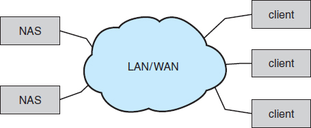
Figure 10.2 Network-attached storage.

Network-attached storage provides a convenient way for all the computers on a LAN to share a pool of storage with the same ease of naming and access enjoyed with local host-attached storage. However, it tends to be less efficient and have lower performance than some direct-attached storage options.

iSCSI is the latest network-attached storage protocol. In essence, it uses the IP network protocol to carry the SCSI protocol. Thus, networks—rather than SCSI cables—can be used as the interconnects between hosts and their storage. As a result, hosts can treat their storage as if it were directly attached, even if the storage is distant from the host.

10.3.3 Storage-Area Network

One drawback of network-attached storage systems is that the storage I/O operations consume bandwidth on the data network, thereby increasing the latency of network communication. This problem can be particularly acute in large client–server installations—the communication between servers and clients competes for bandwidth with the communication among servers and storage devices.

A storage-area network (SAN) is a private network (using storage protocols rather than networking protocols) connecting servers and storage units, as shown in Figure 10.3. The power of a SAN lies in its flexibility. Multiple hosts and multiple storage arrays can attach to the same SAN, and storage can be dynamically allocated to hosts. A SAN switch allows or prohibits access between the hosts and the storage. As one example, if a host is running low on disk space, the SAN can be configured to allocate more storage to that host. SANs make it possible for clusters of servers to share the same storage and for storage arrays to include multiple direct host connections. SANs typically have more ports—as well as more expensive ports—than storage arrays.

FC is the most common SAN interconnect, although the simplicity of iSCSI is increasing its use. Another SAN interconnect is InfiniBand — a special-purpose bus architecture that provides hardware and software support for high-speed interconnection networks for servers and storage units.

10.4 Disk Scheduling

One of the responsibilities of the operating system is to use the hardware efficiently. For the disk drives, meeting this responsibility entails having fast access time and large disk bandwidth. For magnetic disks, the access time has two major components, as mentioned in Section 10.1.1. The seek time is the time for the disk arm to move the heads to the cylinder containing the desired sector. The rotational latency is the additional time for the disk to rotate the desired sector to the disk head. The disk bandwidth is the total number of bytes transferred, divided by the total time between the first request for service and the completion of the last transfer. We can improve both the access time and the bandwidth by managing the order in which disk I/O requests are serviced.

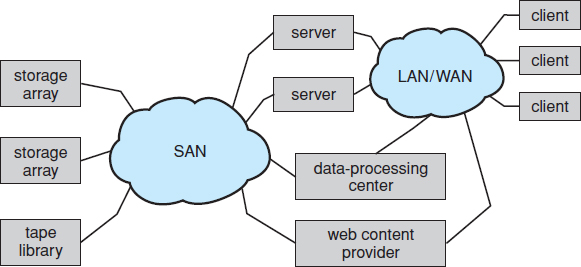
Figure 10.3 Storage-area network

Whenever a process needs I/O to or from the disk, it issues a system call to the operating system. The request specifies several pieces of information:

• Whether this operation is input or output
• What the disk address for the transfer is
• What the memory address for the transfer is
• What the number of sectors to be transferred is

If the desired disk drive and controller are available, the request can be serviced immediately. If the drive or controller is busy, any new requests for service will be placed in the queue of pending requests for that drive. For a multiprogramming system with many processes, the disk queue may often have several pending requests. Thus, when one request is completed, the operating system chooses which pending request to service next. How does the operating system make this choice? Any one of several disk-scheduling algorithms can be used, and we discuss them next.

10.4.1 FCFS Scheduling

The simplest form of disk scheduling is, of course, the first-come, first-served (FCFS) algorithm. This algorithm is intrinsically fair, but it generally does not provide the fastest service. Consider, for example, a disk queue with requests for I/O to blocks on cylinders

98, 183, 37, 122, 14, 124, 65, 67,

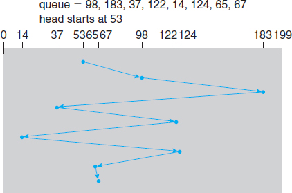
Figure 10.4 FCFS disk scheduling.

in that order. If the disk head is initially at cylinder 53, it will first move from 53 to 98, then to 183, 37, 122, 14, 124, 65, and finally to 67, for a total head movement of 640 cylinders. This schedule is diagrammed in Figure 10.4.

The wild swing from 122 to 14 and then back to 124 illustrates the problem with this schedule. If the requests for cylinders 37 and 14 could be serviced together, before or after the requests for 122 and 124, the total head movement could be decreased substantially, and performance could be thereby improved.

10.4.2 SSTF Scheduling

It seems reasonable to service all the requests close to the current head position before moving the head far away to service other requests. This assumption is the basis for the shortest-seek-time-first (SSTF) algorithm. The SSTF algorithm selects the request with the least seek time from the current head position. In other words, SSTF chooses the pending request closest to the current head position.

For our example request queue, the closest request to the initial head position (53) is at cylinder 65. Once we are at cylinder 65, the next closest request is at cylinder 67. From there, the request at cylinder 37 is closer than the one at 98, so 37 is served next. Continuing, we service the request at cylinder 14, then 98, 122, 124, and finally 183 (Figure 10.5). This scheduling method results in a total head movement of only 236 cylinders—little more than one-third of the distance needed for FCFS scheduling of this request queue. Clearly, this algorithm gives a substantial improvement in performance.

SSTF scheduling is essentially a form of shortest-job-first (SJF) scheduling; and like SJF scheduling, it may cause starvation of some requests. Remember that requests may arrive at any time. Suppose that we have two requests in the queue, for cylinders 14 and 186, and while the request from 14 is being serviced, a new request near 14 arrives. This new request will be serviced next, making the request at 186 wait. While this request is being serviced, another request close to 14 could arrive. In theory, a continual stream of requests near one another could cause the request for cylinder 186 to wait indefinitely. This scenario becomes increasingly likely as the pending-request queue grows longer.

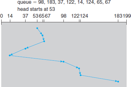
Figure 10.5 SSTF disk scheduling.

Although the SSTF algorithm is a substantial improvement over the FCFS algorithm, it is not optimal. In the example, we can do better by moving the head from 53 to 37, even though the latter is not closest, and then to 14, before turning around to service 65, 67, 98, 122, 124, and 183. This strategy reduces the total head movement to 208 cylinders.

10.4.3 SCAN Scheduling

In the SCAN algorithm, the disk arm starts at one end of the disk and moves toward the other end, servicing requests as it reaches each cylinder, until it gets to the other end of the disk. At the other end, the direction of head movement is reversed, and servicing continues. The head continuously scans back and forth across the disk. The SCAN algorithm is sometimes called the elevator algorithm, since the disk arm behaves just like an elevator in a building, first servicing all the requests going up and then reversing to service requests the other way.

Let's return to our example to illustrate. Before applying SCAN to schedule the requests on cylinders 98, 183, 37, 122, 14, 124, 65, and 67, we need to know the direction of head movement in addition to the head's current position. Assuming that the disk arm is moving toward 0 and that the initial head position is again 53, the head will next service 37 and then 14. At cylinder 0, the arm will reverse and will move toward the other end of the disk, servicing the requests at 65, 67, 98, 122, 124, and 183 (Figure 10.6). If a request arrives in the queue just in front of the head, it will be serviced almost immediately; a request arriving just behind the head will have to wait until the arm moves to the end of the disk, reverses direction, and comes back.

Assuming a uniform distribution of requests for cylinders, consider the density of requests when the head reaches one end and reverses direction. At this point, relatively few requests are immediately in front of the head, since these cylinders have recently been serviced. The heaviest density of requests is at the other end of the disk. These requests have also waited the longest, so why not go there first? That is the idea of the next algorithm.

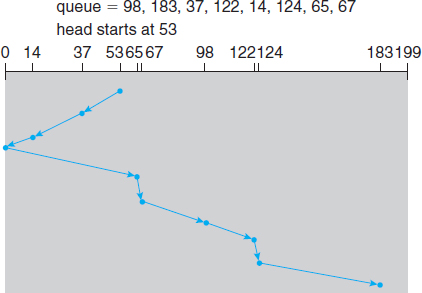
Figure 10.6 SCAN disk scheduling.

10.4.4 C-SCAN Scheduling

Circular SCAN (C-SCAN) scheduling is a variant of SCAN designed to provide a more uniform wait time. Like SCAN, C-SCAN moves the head from one end of the disk to the other, servicing requests along the way. When the head reaches the other end, however, it immediately returns to the beginning of the disk without servicing any requests on the return trip (Figure 10.7). The C-SCAN scheduling algorithm essentially treats the cylinders as a circular list that wraps around from the final cylinder to the first one.

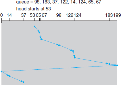
Figure 10.7 C-SCAN disk scheduling.

10.4.5 LOOK Scheduling

As we described them, both SCAN and C-SCAN move the disk arm across the full width of the disk. In practice, neither algorithm is often implemented this way. More commonly, the arm goes only as far as the final request in each direction. Then, it reverses direction immediately, without going all the way to the end of the disk. Versions of SCAN and C-SCAN that follow this pattern are called LOOK and C-LOOK scheduling, because they look for a request before continuing to move in a given direction (Figure 10.8).

10.4.6 Selection of a Disk-Scheduling Algorithm

Given so many disk-scheduling algorithms, how do we choose the best one? SSTF is common and has a natural appeal because it increases performance over FCFS. SCAN and C-SCAN perform better for systems that place a heavy load on the disk, because they are less likely to cause a starvation problem. For any particular list of requests, we can define an optimal order of retrieval, but the computation needed to find an optimal schedule may not justify the savings over SSTF or SCAN. With any scheduling algorithm, however, performance depends heavily on the number and types of requests. For instance, suppose that the queue usually has just one outstanding request. Then, all scheduling algorithms behave the same, because they have only one choice of where to move the disk head: they all behave like FCFS scheduling.

Requests for disk service can be greatly influenced by the file-allocation method. A program reading a contiguously allocated file will generate several requests that are close together on the disk, resulting in limited head movement. A linked or indexed file, in contrast, may include blocks that are widely scattered on the disk, resulting in greater head movement.

The location of directories and index blocks is also important. Since every file must be opened to be used, and opening a file requires searching the directory structure, the directories will be accessed frequently. Suppose that a directory entry is on the first cylinder and a file's data are on the final cylinder. In this case, the disk head has to move the entire width of the disk. If the directory entry were on the middle cylinder, the head would have to move only one-half the width. Caching the directories and index blocks in main memory can also help to reduce disk-arm movement, particularly for read requests.

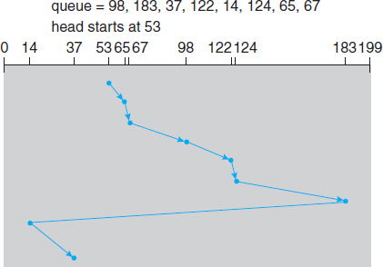
Figure 10.8 C-LOOK disk scheduling.

Because of these complexities, the disk-scheduling algorithm should be written as a separate module of the operating system, so that it can be replaced with a different algorithm if necessary. Either SSTF or LOOK is a reasonable choice for the default algorithm.

The scheduling algorithms described here consider only the seek distances. For modern disks, the rotational latency can be nearly as large as the average seek time. It is difficult for the operating system to schedule for improved rotational latency, though, because modern disks do not disclose the physical location of logical blocks. Disk manufacturers have been alleviating this problem by implementing disk-scheduling algorithms in the controller hardware built into the disk drive. If the operating system sends a batch of requests to the controller, the controller can queue them and then schedule them to improve both the seek time and the rotational latency.

If I/O performance were the only consideration, the operating system would gladly turn over the responsibility of disk scheduling to the disk hardware. In practice, however, the operating system may have other constraints on the service order for requests. For instance, demand paging may take priority over application I/O, and writes are more urgent than reads if the cache is running out of free pages. Also, it may be desirable to guarantee the order of a set of disk writes to make the file system robust in the face of system crashes. Consider what could happen if the operating system allocated a disk page to a file and the application wrote data into that page before the operating system had a chance to flush the file system metadata back to disk. To accommodate such requirements, an operating system may choose to do its own disk scheduling and to spoon-feed the requests to the disk controller, one by one, for some types of I/O.

10.5 Disk Management

The operating system is responsible for several other aspects of disk management, too. Here we discuss disk initialization, booting from disk, and bad-block recovery.

10.5.1 Disk Formatting

A new magnetic disk is a blank slate: it is just a platter of a magnetic recording material. Before a disk can store data, it must be divided into sectors that the disk controller can read and write. This process is called low-level formatting, or physical formatting. Low-level formatting fills the disk with a special data structure for each sector. The data structure for a sector typically consists of a header, a data area (usually 512 bytes in size), and a trailer. The header and trailer contain information used by the disk controller, such as a sector number and an error-correcting code (ECC). When the controller writes a sector of data during normal I/O, the ECC is updated with a value calculated from all the bytes in the data area. When the sector is read, the ECC is recalculated and compared with the stored value. If the stored and calculated numbers are different, this mismatch indicates that the data area of the sector has become corrupted and that the disk sector may be bad (Section 10.5.3). The ECC is an error-correcting code because it contains enough information, if only a few bits of data have been corrupted, to enable the controller to identify which bits have changed and calculate what their correct values should be. It then reports a recoverable soft error. The controller automatically does the ECC processing whenever a sector is read or written.

Most hard disks are low-level-formatted at the factory as a part of the manufacturing process. This formatting enables the manufacturer to test the disk and to initialize the mapping from logical block numbers to defect-free sectors on the disk. For many hard disks, when the disk controller is instructed to low-level-format the disk, it can also be told how many bytes of data space to leave between the header and trailer of all sectors. It is usually possible to choose among a few sizes, such as 256, 512, and 1,024 bytes. Formatting a disk with a larger sector size means that fewer sectors can fit on each track; but it also means that fewer headers and trailers are written on each track and more space is available for user data. Some operating systems can handle only a sector size of 512 bytes.

Before it can use a disk to hold files, the operating system still needs to record its own data structures on the disk. It does so in two steps. The first step is to partition the disk into one or more groups of cylinders. The operating system can treat each partition as though it were a separate disk. For instance, one partition can hold a copy of the operating system's executable code, while another holds user files. The second step is logical formatting, or creation of a file system. In this step, the operating system stores the initial file-system data structures onto the disk. These data structures may include maps of free and allocated space and an initial empty directory.

To increase efficiency, most file systems group blocks together into larger chunks, frequently called clusters. Disk I/O is done via blocks, but file system I/O is done via clusters, effectively assuring that I/O has more sequential-access and fewer random-access characteristics.

Some operating systems give special programs the ability to use a disk partition as a large sequential array of logical blocks, without any file-system data structures. This array is sometimes called the raw disk, and I/O to this array is termed raw I/O. For example, some database systems prefer raw I/O because it enables them to control the exact disk location where each database record is stored. Raw I/O bypasses all the file-system services, such as the buffer cache, file locking, prefetching, space allocation, file names, and directories. We can make certain applications more efficient by allowing them to implement their own special-purpose storage services on a raw partition, but most applications perform better when they use the regular file-system services.

10.5.2 Boot Block

For a computer to start running—for instance, when it is powered up or rebooted—it must have an initial program to run. This initial bootstrap program tends to be simple. It initializes all aspects of the system, from CPU registers to device controllers and the contents of main memory, and then starts the operating system. To do its job, the bootstrap program finds the operating-system kernel on disk, loads that kernel into memory, and jumps to an initial address to begin the operating-system execution.

For most computers, the bootstrap is stored in read-only memory (ROM). This location is convenient, because ROM needs no initialization and is at a fixed location that the processor can start executing when powered up or reset. And, since ROM is read only, it cannot be infected by a computer virus. The problem is that changing this bootstrap code requires changing the ROM hardware chips. For this reason, most systems store a tiny bootstrap loader program in the boot ROM whose only job is to bring in a full bootstrap program from disk. The full bootstrap program can be changed easily: a new version is simply written onto the disk. The full bootstrap program is stored in the “boot blocks” at a fixed location on the disk. A disk that has a boot partition is called a boot disk or system disk.

The code in the boot ROM instructs the disk controller to read the boot blocks into memory (no device drivers are loaded at this point) and then starts executing that code. The full bootstrap program is more sophisticated than the bootstrap loader in the boot ROM. It is able to load the entire operating system from a non-fixed location on disk and to start the operating system running. Even so, the full bootstrap code may be small.

Let's consider as an example the boot process in Windows. First, note that Windows allows a hard disk to be divided into partitions, and one partition—identified as the boot partition—contains the operating system and device drivers. The Windows system places its boot code in the first sector on the hard disk, which it terms the master boot record, or MBR. Booting begins by running code that is resident in the system's ROM memory. This code directs the system to read the boot code from the MBR. In addition to containing boot code, the MBR contains a table listing the partitions for the hard disk and a flag indicating which partition the system is to be booted from, as illustrated in Figure 10.9. Once the system identifies the boot partition, it reads the first sector from that partition (which is called the boot sector) and continues with the remainder of the boot process, which includes loading the various subsystems and system services.

10.5.3 Bad Blocks

Because disks have moving parts and small tolerances (recall that the disk head flies just above the disk surface), they are prone to failure. Sometimes the failure is complete; in this case, the disk needs to be replaced and its contents restored from backup media to the new disk. More frequently, one or more sectors become defective. Most disks even come from the factory with bad blocks. Depending on the disk and controller in use, these blocks are handled in a variety of ways.

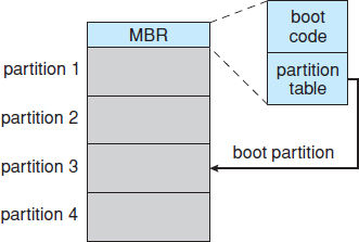
Figure 10.9 Booting from disk in Windows.

On simple disks, such as some disks with IDE controllers, bad blocks are handled manually. One strategy is to scan the disk to find bad blocks while the disk is being formatted. Any bad blocks that are discovered are flagged as unusable so that the file system does not allocate them. If blocks go bad during normal operation, a special program (such as the Linux badblocks command) must be run manually to search for the bad blocks and to lock them away. Data that resided on the bad blocks usually are lost.

More sophisticated disks are smarter about bad-block recovery. The controller maintains a list of bad blocks on the disk. The list is initialized during the low-level formatting at the factory and is updated over the life of the disk. Low-level formatting also sets aside spare sectors not visible to the operating system. The controller can be told to replace each bad sector logically with one of the spare sectors. This scheme is known as sector sparing or forwarding.

A typical bad-sector transaction might be as follows:

• The operating system tries to read logical block 87.
• The controller calculates the ECC and finds that the sector is bad. It reports this finding to the operating system.
• The next time the system is rebooted, a special command is run to tell the controller to replace the bad sector with a spare.
• After that, whenever the system requests logical block 87, the request is translated into the replacement sector's address by the controller.

Note that such a redirection by the controller could invalidate any optimization by the operating system's disk-scheduling algorithm! For this reason, most disks are formatted to provide a few spare sectors in each cylinder and a spare cylinder as well. When a bad block is remapped, the controller uses a spare sector from the same cylinder, if possible.

As an alternative to sector sparing, some controllers can be instructed to replace a bad block by sector slipping. Here is an example: Suppose that logical block 17 becomes defective and the first available spare follows sector 202. Sector slipping then remaps all the sectors from 17 to 202, moving them all down one spot. That is, sector 202 is copied into the spare, then sector 201 into 202, then 200 into 201, and so on, until sector 18 is copied into sector 19. Slipping the sectors in this way frees up the space of sector 18 so that sector 17 can be mapped to it.

The replacement of a bad block generally is not totally automatic, because the data in the bad block are usually lost. Soft errors may trigger a process in which a copy of the block data is made and the block is spared or slipped. An unrecoverable hard error, however, results in lost data. Whatever file was using that block must be repaired (for instance, by restoration from a backup tape), and that requires manual intervention.

10.6 Swap-Space Management

Swapping was first presented in Section 8.2, where we discussed moving entire processes between disk and main memory. Swapping in that setting occurs when the amount of physical memory reaches a critically low point and processes are moved from memory to swap space to free available memory. In practice, very few modern operating systems implement swapping in this fashion. Rather, systems now combine swapping with virtual memory techniques (Chapter 9) and swap pages, not necessarily entire processes. In fact, some systems now use the terms “swapping” and “paging” interchangeably, reflecting the merging of these two concepts.

Swap-space management is another low-level task of the operating system. Virtual memory uses disk space as an extension of main memory. Since disk access is much slower than memory access, using swap space significantly decreases system performance. The main goal for the design and implementation of swap space is to provide the best throughput for the virtual memory system. In this section, we discuss how swap space is used, where swap space is located on disk, and how swap space is managed.

10.6.1 Swap-Space Use

Swap space is used in various ways by different operating systems, depending on the memory-management algorithms in use. For instance, systems that implement swapping may use swap space to hold an entire process image, including the code and data segments. Paging systems may simply store pages that have been pushed out of main memory. The amount of swap space needed on a system can therefore vary from a few megabytes of disk space to gigabytes, depending on the amount of physical memory, the amount of virtual memory it is backing, and the way in which the virtual memory is used.

Note that it may be safer to overestimate than to underestimate the amount of swap space required, because if a system runs out of swap space it may be forced to abort processes or may crash entirely. Overestimation wastes disk space that could otherwise be used for files, but it does no other harm. Some systems recommend the amount to be set aside for swap space. Solaris, for example, suggests setting swap space equal to the amount by which virtual memory exceeds pageable physical memory. In the past, Linux has suggested setting swap space to double the amount of physical memory. Today, that limitation is gone, and most Linux systems use considerably less swap space.

Some operating systems—including Linux—allow the use of multiple swap spaces, including both files and dedicated swap partitions. These swap spaces are usually placed on separate disks so that the load placed on the I/O system by paging and swapping can be spread over the system's I/O bandwidth.

10.6.2 Swap-Space Location

A swap space can reside in one of two places: it can be carved out of the normal file system, or it can be in a separate disk partition. If the swap space is simply a large file within the file system, normal file-system routines can be used to create it, name it, and allocate its space. This approach, though easy to implement, is inefficient. Navigating the directory structure and the disk-allocation data structures takes time and (possibly) extra disk accesses. External fragmentation can greatly increase swapping times by forcing multiple seeks during reading or writing of a process image. We can improve performance by caching the block location information in physical memory and by using special tools to allocate physically contiguous blocks for the swap file, but the cost of traversing the file-system data structures remains.

Alternatively, swap space can be created in a separate raw partition. No file system or directory structure is placed in this space. Rather, a separate swap-space storage manager is used to allocate and deallocate the blocks from the raw partition. This manager uses algorithms optimized for speed rather than for storage efficiency, because swap space is accessed much more frequently than file systems (when it is used). Internal fragmentation may increase, but this trade-off is acceptable because the life of data in the swap space generally is much shorter than that of files in the file system. Since swap space is reinitialized at boot time, any fragmentation is short-lived. The raw-partition approach creates a fixed amount of swap space during disk partitioning. Adding more swap space requires either repartitioning the disk (which involves moving the other file-system partitions or destroying them and restoring them from backup) or adding another swap space elsewhere.

Some operating systems are flexible and can swap both in raw partitions and in file-system space. Linux is an example: the policy and implementation are separate, allowing the machine's administrator to decide which type of swapping to use. The trade-off is between the convenience of allocation and management in the file system and the performance of swapping in raw partitions.

10.6.3 Swap-Space Management: An Example

We can illustrate how swap space is used by following the evolution of swapping and paging in various UNIX systems. The traditional UNIX kernel started with an implementation of swapping that copied entire processes between contiguous disk regions and memory. UNIX later evolved to a combination of swapping and paging as paging hardware became available.

In Solaris 1 (SunOS), the designers changed standard UNIX methods to improve efficiency and reflect technological developments. When a process executes, text-segment pages containing code are brought in from the file system, accessed in main memory, and thrown away if selected for pageout. It is more efficient to reread a page from the file system than to write it to swap space and then reread it from there. Swap space is only used as a backing store for pages of anonymous memory, which includes memory allocated for the stack, heap, and uninitialized data of a process.

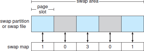
Figure 10.10 The data structures for swapping on Linux systems.

More changes were made in later versions of Solaris. The biggest change is that Solaris now allocates swap space only when a page is forced out of physical memory, rather than when the virtual memory page is first created. This scheme gives better performance on modern computers, which have more physical memory than older systems and tend to page less.

Linux is similar to Solaris in that swap space is used only for anonymous memory—that is, memory not backed by any file. Linux allows one or more swap areas to be established. A swap area may be in either a swap file on a regular file system or a dedicated swap partition. Each swap area consists of a series of 4-KB page slots, which are used to hold swapped pages. Associated with each swap area is a swap map—an array of integer counters, each corresponding to a page slot in the swap area. If the value of a counter is 0, the corresponding page slot is available. Values greater than 0 indicate that the page slot is occupied by a swapped page. The value of the counter indicates the number of mappings to the swapped page. For example, a value of 3 indicates that the swapped page is mapped to three different processes (which can occur if the swapped page is storing a region of memory shared by three processes). The data structures for swapping on Linux systems are shown in Figure 10.10.

10.7 RAID Structure

Disk drives have continued to get smaller and cheaper, so it is now economically feasible to attach many disks to a computer system. Having a large number of disks in a system presents opportunities for improving the rate at which data can be read or written, if the disks are operated in parallel. Furthermore, this setup offers the potential for improving the reliability of data storage, because redundant information can be stored on multiple disks. Thus, failure of one disk does not lead to loss of data. A variety of disk-organization techniques, collectively called redundant arrays of independent disks (RAID), are commonly used to address the performance and reliability issues.

In the past, RAIDs composed of small, cheap disks were viewed as a cost-effective alternative to large, expensive disks. Today, RAIDs are used for their higher reliability and higher data-transfer rate, rather than for economic reasons. Hence, the I in RAID, which once stood for “inexpensive,” now stands for “independent.”

10.7.1 Improvement of Reliability via Redundancy

Let's first consider the reliability of RAIDs. The chance that some disk out of a set of N disks will fail is much higher than the chance that a specific single disk will fail. Suppose that the mean time to failure of a single disk is 100,000 hours. Then the mean time to failure of some disk in an array of 100 disks will be 100,000/100 = 1,000 hours, or 41.66 days, which is not long at all! If we store only one copy of the data, then each disk failure will result in loss of a significant amount of data—and such a high rate of data loss is unacceptable.

The solution to the problem of reliability is to introduce redundancy; we store extra information that is not normally needed but that can be used in the event of failure of a disk to rebuild the lost information. Thus, even if a disk fails, data are not lost.

The simplest (but most expensive) approach to introducing redundancy is to duplicate every disk. This technique is called mirroring. With mirroring, a logical disk consists of two physical disks, and every write is carried out on both disks. The result is called a mirrored volume. If one of the disks in the volume fails, the data can be read from the other. Data will be lost only if the second disk fails before the first failed disk is replaced.

The mean time to failure of a mirrored volume—where failure is the loss of data—depends on two factors. One is the mean time to failure of the individual disks. The other is the mean time to repair, which is the time it takes (on average) to replace a failed disk and to restore the data on it. Suppose that the failures of the two disks are independent; that is, the failure of one disk is not connected to the failure of the other. Then, if the mean time to failure of a single disk is 100,000 hours and the mean time to repair is 10 hours, the mean time to data loss of a mirrored disk system is 100,000²/(2 * 10) = 500 * 10⁶ hours, or 57,000 years!

You should be aware that we cannot really assume that disk failures will be independent. Power failures and natural disasters, such as earthquakes, fires, and floods, may result in damage to both disks at the same time. Also, manufacturing defects in a batch of disks can cause correlated failures. As disks age, the probability of failure grows, increasing the chance that a second disk will fail while the first is being repaired. In spite of all these considerations, however, mirrored-disk systems offer much higher reliability than do single-disk systems.

Power failures are a particular source of concern, since they occur far more frequently than do natural disasters. Even with mirroring of disks, if writes are in progress to the same block in both disks, and power fails before both blocks are fully written, the two blocks can be in an inconsistent state. One solution to this problem is to write one copy first, then the next. Another is to add a solid-state nonvolatile RAM (NVRAM) cache to the RAID array. This write-back cache is protected from data loss during power failures, so the write can be considered complete at that point, assuming the NVRAM has some kind of error protection and correction, such as ECC or mirroring.

10.7.2 Improvement in Performance via Parallelism

Now let's consider how parallel access to multiple disks improves performance. With disk mirroring, the rate at which read requests can be handled is doubled, since read requests can be sent to either disk (as long as both disks in a pair are functional, as is almost always the case). The transfer rate of each read is the same as in a single-disk system, but the number of reads per unit time has doubled.

With multiple disks, we can improve the transfer rate as well (or instead) by striping data across the disks. In its simplest form, data striping consists of splitting the bits of each byte across multiple disks; such striping is called bit-level striping. For example, if we have an array of eight disks, we write bit i of each byte to disk i. The array of eight disks can be treated as a single disk with sectors that are eight times the normal size and, more important, that have eight times the access rate. Every disk participates in every access (read or write); so the number of accesses that can be processed per second is about the same as on a single disk, but each access can read eight times as many data in the same time as on a single disk.

Bit-level striping can be generalized to include a number of disks that either is a multiple of 8 or divides 8. For example, if we use an array of four disks, bits i and 4 + i of each byte go to disk i. Further, striping need not occur at the bit level. In block-level striping, for instance, blocks of a file are striped across multiple disks; with n disks, block i of a file goes to disk (i mod n) + 1. Other levels of striping, such as bytes of a sector or sectors of a block, also are possible. Block-level striping is the most common.

Parallelism in a disk system, as achieved through striping, has two main goals:

1. Increase the throughput of multiple small accesses (that is, page accesses) by load balancing.
2. Reduce the response time of large accesses.

10.7.3 RAID Levels

Mirroring provides high reliability, but it is expensive. Striping provides high data-transfer rates, but it does not improve reliability. Numerous schemes to provide redundancy at lower cost by using disk striping combined with “parity” bits (which we describe shortly) have been proposed. These schemes have different cost–performance trade-offs and are classified according to levels called RAID levels. We describe the various levels here; Figure 10.11 shows them pictorially (in the figure, P indicates error-correcting bits and C indicates a second copy of the data). In all cases depicted in the figure, four disks' worth of data are stored, and the extra disks are used to store redundant information for failure recovery.

Figure 10.11 RAID levels.

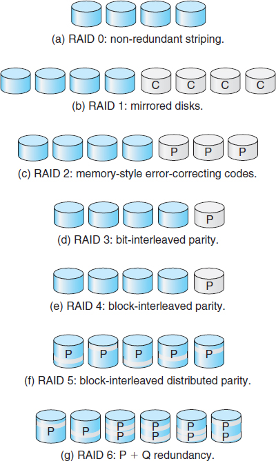
• RAID level 0. RAID level 0 refers to disk arrays with striping at the level of blocks but without any redundancy (such as mirroring or parity bits), as shown in Figure 10.11(a).
• RAID level 1. RAID level 1 refers to disk mirroring. Figure 10.11(b) shows a mirrored organization.
• RAID level 2. RAID level 2 is also known as memory-style error-correcting-code (ECC) organization. Memory systems have long detected certain errors by using parity bits. Each byte in a memory system may have a parity bit associated with it that records whether the number of bits in the byte set to 1 is even (parity = 0) or odd (parity = 1). If one of the bits in the byte is damaged (either a 1 becomes a 0, or a 0 becomes a 1), the parity of the byte changes and thus does not match the stored parity. Similarly, if the stored parity bit is damaged, it does not match the computed parity. Thus, all single-bit errors are detected by the memory system. Error-correcting schemes store two or more extra bits and can reconstruct the data if a single bit is damaged.

  The idea of ECC can be used directly in disk arrays via striping of bytes across disks. For example, the first bit of each byte can be stored in disk 1, the second bit in disk 2, and so on until the eighth bit is stored in disk 8; the error-correction bits are stored in further disks. This scheme is shown in Figure 10.11(c), where the disks labeled P store the error-correction bits. If one of the disks fails, the remaining bits of the byte and the associated error-correction bits can be read from other disks and used to reconstruct the damaged data. Note that RAID level 2 requires only three disks' overhead for four disks of data, unlike RAID level 1, which requires four disks' overhead.

• RAID level 3. RAID level 3, or bit-interleaved parity organization, improves on level 2 by taking into account the fact that, unlike memory systems, disk controllers can detect whether a sector has been read correctly, so a single parity bit can be used for error correction as well as for detection. The idea is as follows: If one of the sectors is damaged, we know exactly which sector it is, and we can figure out whether any bit in the sector is a 1 or a 0 by computing the parity of the corresponding bits from sectors in the other disks. If the parity of the remaining bits is equal to the stored parity, the missing bit is 0; otherwise, it is 1. RAID level 3 is as good as level 2 but is less expensive in the number of extra disks required (it has only a one-disk overhead), so level 2 is not used in practice. Level 3 is shown pictorially in Figure 10.11(d).

  RAID level 3 has two advantages over level 1. First, the storage overhead is reduced because only one parity disk is needed for several regular disks, whereas one mirror disk is needed for every disk in level 1. Second, since reads and writes of a byte are spread out over multiple disks with N-way striping of data, the transfer rate for reading or writing a single block is N times as fast as with RAID level 1. On the negative side, RAID level 3 supports fewer I/Os per second, since every disk has to participate in every I/O request.

  A further performance problem with RAID 3—and with all parity-based RAID levels—is the expense of computing and writing the parity. This overhead results in significantly slower writes than with non-parity RAID arrays. To moderate this performance penalty, many RAID storage arrays include a hardware controller with dedicated parity hardware. This controller offloads the parity computation from the CPU to the array. The array has an NVRAM cache as well, to store the blocks while the parity is computed and to buffer the writes from the controller to the spindles. This combination can make parity RAID almost as fast as non-parity. In fact, a caching array doing parity RAID can outperform a non-caching non-parity RAID.

• RAID level 4. RAID level 4, or block-interleaved parity organization, uses block-level striping, as in RAID 0, and in addition keeps a parity block on a separate disk for corresponding blocks from N other disks. This scheme is diagrammed in Figure 10.11(e). If one of the disks fails, the parity block can be used with the corresponding blocks from the other disks to restore the blocks of the failed disk.

  A block read accesses only one disk, allowing other requests to be processed by the other disks. Thus, the data-transfer rate for each access is slower, but multiple read accesses can proceed in parallel, leading to a higher overall I/O rate. The transfer rates for large reads are high, since all the disks can be read in parallel. Large writes also have high transfer rates, since the data and parity can be written in parallel.

  Small independent writes cannot be performed in parallel. An operating-system write of data smaller than a block requires that the block be read, modified with the new data, and written back. The parity block has to be updated as well. This is known as the read-modify-write cycle. Thus, a single write requires four disk accesses: two to read the two old blocks and two to write the two new blocks.

  WAFL (which we cover in Chapter 12) uses RAID level 4 because this RAID level allows disks to be added to a RAID set seamlessly. If the added disks are initialized with blocks containing only zeros, then the parity value does not change, and the RAID set is still correct.

• RAID level 5. RAID level 5, or block-interleaved distributed parity, differs from level 4 in that it spreads data and parity among all N+1 disks, rather than storing data in N disks and parity in one disk. For each block, one of the disks stores the parity and the others store data. For example, with an array of five disks, the parity for the nth block is stored in disk (n mod 5)+1. The nth blocks of the other four disks store actual data for that block. This setup is shown in Figure 10.11(f), where the Ps are distributed across all the disks. A parity block cannot store parity for blocks in the same disk, because a disk failure would result in loss of data as well as of parity, and hence the loss would not be recoverable. By spreading the parity across all the disks in the set, RAID 5 avoids potential overuse of a single parity disk, which can occur with RAID 4. RAID 5 is the most common parity RAID system.
• RAID level 6. RAID level 6, also called the P + Q redundancy scheme, is much like RAID level 5 but stores extra redundant information to guard against multiple disk failures. Instead of parity, error-correcting codes such as the Reed–Solomon codes are used. In the scheme shown in Figure 10.11(g), 2 bits of redundant data are stored for every 4 bits of data—compared with 1 parity bit in level 5—and the system can tolerate two disk failures.
• RAID levels 0 + 1 and 1 + 0. RAID level 0 + 1 refers to a combination of RAID levels 0 and 1. RAID 0 provides the performance, while RAID 1 provides the reliability. Generally, this level provides better performance than RAID 5. It is common in environments where both performance and reliability are important. Unfortunately, like RAID 1, it doubles the number of disks needed for storage, so it is also relatively expensive. In RAID 0 + 1, a set of disks are striped, and then the stripe is mirrored to another, equivalent stripe.

  Another RAID option that is becoming available commercially is RAID level 1 + 0, in which disks are mirrored in pairs and then the resulting mirrored pairs are striped. This scheme has some theoretical advantages over RAID 0 + 1. For example, if a single disk fails in RAID 0 + 1, an entire stripe is inaccessible, leaving only the other stripe. With a failure in RAID 1 + 0, a single disk is unavailable, but the disk that mirrors it is still available, as are all the rest of the disks (Figure 10.12).

Numerous variations have been proposed to the basic RAID schemes described here. As a result, some confusion may exist about the exact definitions of the different RAID levels.

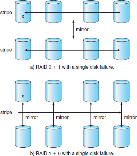
Figure 10.12 RAID 0 + 1 and 1 + 0.

The implementation of RAID is another area of variation. Consider the following layers at which RAID can be implemented.

• Volume-management software can implement RAID within the kernel or at the system software layer. In this case, the storage hardware can provide minimal features and still be part of a full RAID solution. Parity RAID is fairly slow when implemented in software, so typically RAID 0, 1, or 0 + 1 is used.
• RAID can be implemented in the host bus-adapter (HBA) hardware. Only the disks directly connected to the HBA can be part of a given RAID set. This solution is low in cost but not very flexible.
• RAID can be implemented in the hardware of the storage array. The storage array can create RAID sets of various levels and can even slice these sets into smaller volumes, which are then presented to the operating system. The operating system need only implement the file system on each of the volumes. Arrays can have multiple connections available or can be part of a SAN, allowing multiple hosts to take advantage of the array's features.
• RAID can be implemented in the SAN interconnect layer by disk virtualization devices. In this case, a device sits between the hosts and the storage. It accepts commands from the servers and manages access to the storage. It could provide mirroring, for example, by writing each block to two separate storage devices.

Other features, such as snapshots and replication, can be implemented at each of these levels as well. A snapshot is a view of the file system before the last update took place. (Snapshots are covered more fully in Chapter 12.) Replication involves the automatic duplication of writes between separate sites for redundancy and disaster recovery. Replication can be synchronous or asynchronous. In synchronous replication, each block must be written locally and remotely before the write is considered complete, whereas in asynchronous replication, the writes are grouped together and written periodically. Asynchronous replication can result in data loss if the primary site fails, but it is faster and has no distance limitations.

The implementation of these features differs depending on the layer at which RAID is implemented. For example, if RAID is implemented in software, then each host may need to carry out and manage its own replication. If replication is implemented in the storage array or in the SAN interconnect, however, then whatever the host operating system or its features, the host's data can be replicated.

One other aspect of most RAID implementations is a hot spare disk or disks. A hot spare is not used for data but is configured to be used as a replacement in case of disk failure. For instance, a hot spare can be used to rebuild a mirrored pair should one of the disks in the pair fail. In this way, the RAID level can be reestablished automatically, without waiting for the failed disk to be replaced. Allocating more than one hot spare allows more than one failure to be repaired without human intervention.

10.7.4 Selecting a RAID Level

Given the many choices they have, how do system designers choose a RAID level? One consideration is rebuild performance. If a disk fails, the time needed to rebuild its data can be significant. This may be an important factor if a continuous supply of data is required, as it is in high-performance or interactive database systems. Furthermore, rebuild performance influences the mean time to failure.

Rebuild performance varies with the RAID level used. Rebuilding is easiest for RAID level 1, since data can be copied from another disk. For the other levels, we need to access all the other disks in the array to rebuild data in a failed disk. Rebuild times can be hours for RAID 5 rebuilds of large disk sets.

RAID level 0 is used in high-performance applications where data loss is not critical. RAID level 1 is popular for applications that require high reliability with fast recovery. RAID 0 + 1 and 1 + 0 are used where both performance and reliability are important—for example, for small databases. Due to RAID 1's high space overhead, RAID 5 is often preferred for storing large volumes of data. Level 6 is not supported currently by many RAID implementations, but it should offer better reliability than level 5.

RAID system designers and administrators of storage have to make several other decisions as well. For example, how many disks should be in a given RAID set? How many bits should be protected by each parity bit? If more disks are in an array, data-transfer rates are higher, but the system is more expensive. If more bits are protected by a parity bit, the space overhead due to parity bits is lower, but the chance that a second disk will fail before the first failed disk is repaired is greater, and that will result in data loss.

10.7.5 Extensions

The concepts of RAID have been generalized to other storage devices, including arrays of tapes, and even to the broadcast of data over wireless systems. When applied to arrays of tapes, RAID structures are able to recover data even if one of the tapes in an array is damaged. When applied to broadcast of data, a block of data is split into short units and is broadcast along with a parity unit. If one of the units is not received for any reason, it can be reconstructed from the other units. Commonly, tape-drive robots containing multiple tape drives will stripe data across all the drives to increase throughput and decrease backup time.

10.7.6 Problems with RAID

Unfortunately, RAID does not always assure that data are available for the operating system and its users. A pointer to a file could be wrong, for example, or pointers within the file structure could be wrong. Incomplete writes, if not properly recovered, could result in corrupt data. Some other process could accidentally write over a file system's structures, too. RAID protects against physical media errors, but not other hardware and software errors. As large as is the landscape of software and hardware bugs, that is how numerous are the potential perils for data on a system.

The Solaris ZFS file system takes an innovative approach to solving these problems through the use of checksums—a technique used to verify the integrity of data. ZFS maintains internal checksums of all blocks, including data and metadata. These checksums are not kept with the block that is being checksummed. Rather, they are stored with the pointer to that block. (See Figure 10.13.) Consider an inode — a data structure for storing file system metadata — with pointers to its data. Within the inode is the checksum of each block of data. If there is a problem with the data, the checksum will be incorrect, and the file system will know about it. If the data are mirrored, and there is a block with a correct checksum and one with an incorrect checksum, ZFS will automatically update the bad block with the good one. Similarly, the directory entry that points to the inode has a checksum for the inode. Any problem in the inode is detected when the directory is accessed. This checksumming takes places throughout all ZFS structures, providing a much higher level of consistency, error detection, and error correction than is found in RAID disk sets or standard file systems. The extra overhead that is created by the checksum calculation and extra block read-modify-write cycles is not noticeable because the overall performance of ZFS is very fast.

Another issue with most RAID implementations is lack of flexibility. Consider a storage array with twenty disks divided into four sets of five disks. Each set of five disks is a RAID level 5 set. As a result, there are four separate volumes, each holding a file system. But what if one file system is too large to fit on a five-disk RAID level 5 set? And what if another file system needs very little space? If such factors are known ahead of time, then the disks and volumes can be properly allocated. Very frequently, however, disk use and requirements change over time.

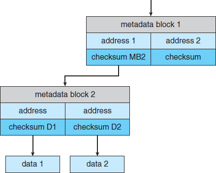
Figure 10.13 ZFS checksums all metadata and data.

Even if the storage array allowed the entire set of twenty disks to be created as one large RAID set, other issues could arise. Several volumes of various sizes could be built on the set. But some volume managers do not allow us to change a volume's size. In that case, we would be left with the same issue described above—mismatched file-system sizes. Some volume managers allow size changes, but some file systems do not allow for file-system growth or shrinkage. The volumes could change sizes, but the file systems would need to be recreated to take advantage of those changes.

ZFS combines file-system management and volume management into a unit providing greater functionality than the traditional separation of those functions allows. Disks, or partitions of disks, are gathered together via RAID sets into pools of storage. A pool can hold one or more ZFS file systems. The entire pool's free space is available to all file systems within that pool. ZFS uses the memory model of malloc() and free() to allocate and release storage for each file system as blocks are used and freed within the file system. As a result, there are no artificial limits on storage use and no need to relocate file systems between volumes or resize volumes. ZFS provides quotas to limit the size of a file system and reservations to assure that a file system can grow by a specified amount, but those variables can be changed by the file-system owner at any time. Figure 10.14(a) depicts traditional volumes and file systems, and Figure 10.14(b) shows the ZFS model.

10.8 Stable-Storage Implementation

In Chapter 5, we introduced the write-ahead log, which requires the availability of stable storage. By definition, information residing in stable storage is never lost. To implement such storage, we need to replicate the required information on multiple storage devices (usually disks) with independent failure modes. We also need to coordinate the writing of updates in a way that guarantees that a failure during an update will not leave all the copies in a damaged state and that, when we are recovering from a failure, we can force all copies to a consistent and correct value, even if another failure occurs during the recovery. In this section, we discuss how to meet these needs.

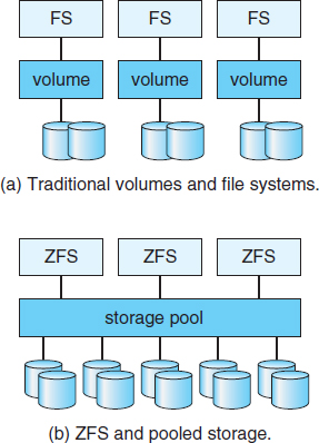
Figure 10.14 (a) Traditional volumes and file systems. (b) A ZFS pool and file systems.

A disk write results in one of three outcomes:

1. Successful completion. The data were written correctly on disk.
2. Partial failure. A failure occurred in the midst of transfer, so only some of the sectors were written with the new data, and the sector being written during the failure may have been corrupted.
3. Total failure. The failure occurred before the disk write started, so the previous data values on the disk remain intact.

Whenever a failure occurs during writing of a block, the system needs to detect it and invoke a recovery procedure to restore the block to a consistent state. To do that, the system must maintain two physical blocks for each logical block. An output operation is executed as follows:

1. Write the information onto the first physical block.
2. When the first write completes successfully, write the same information onto the second physical block.
3. Declare the operation complete only after the second write completes successfully.

During recovery from a failure, each pair of physical blocks is examined. If both are the same and no detectable error exists, then no further action is necessary. If one block contains a detectable error then we replace its contents with the value of the other block. If neither block contains a detectable error, but the blocks differ in content, then we replace the content of the first block with that of the second. This recovery procedure ensures that a write to stable storage either succeeds completely or results in no change.

We can extend this procedure easily to allow the use of an arbitrarily large number of copies of each block of stable storage. Although having a large number of copies further reduces the probability of a failure, it is usually reasonable to simulate stable storage with only two copies. The data in stable storage are guaranteed to be safe unless a failure destroys all the copies.

Because waiting for disk writes to complete (synchronous I/O) is time consuming, many storage arrays add NVRAM as a cache. Since the memory is nonvolatile (it usually has battery power to back up the unit's power), it can be trusted to store the data en route to the disks. It is thus considered part of the stable storage. Writes to it are much faster than to disk, so performance is greatly improved.

10.9 Summary

Disk drives are the major secondary storage I/O devices on most computers. Most secondary storage devices are either magnetic disks or magnetic tapes, although solid-state disks are growing in importance. Modern disk drives are structured as large one-dimensional arrays of logical disk blocks. Generally, these logical blocks are 512 bytes in size. Disks may be attached to a computer system in one of two ways: (1) through the local I/O ports on the host computer or (2) through a network connection.

Requests for disk I/O are generated by the file system and by the virtual memory system. Each request specifies the address on the disk to be referenced, in the form of a logical block number. Disk-scheduling algorithms can improve the effective bandwidth, the average response time, and the variance in response time. Algorithms such as SSTF, SCAN, C-SCAN, LOOK, and C-LOOK are designed to make such improvements through strategies for disk-queue ordering. Performance of disk-scheduling algorithms can vary greatly on magnetic disks. In contrast, because solid-state disks have no moving parts, performance varies little among algorithms, and quite often a simple FCFS strategy is used.

Performance can be harmed by external fragmentation. Some systems have utilities that scan the file system to identify fragmented files; they then move blocks around to decrease the fragmentation. Defragmenting a badly fragmented file system can significantly improve performance, but the system may have reduced performance while the defragmentation is in progress. Sophisticated file systems, such as the UNIX Fast File System, incorporate many strategies to control fragmentation during space allocation so that disk reorganization is not needed.

The operating system manages the disk blocks. First, a disk must be low-level-formatted to create the sectors on the raw hardware—new disks usually come preformatted. Then, the disk is partitioned, file systems are created, and boot blocks are allocated to store the system's bootstrap program. Finally, when a block is corrupted, the system must have a way to lock out that block or to replace it logically with a spare.

Because an efficient swap space is a key to good performance, systems usually bypass the file system and use raw-disk access for paging I/O. Some systems dedicate a raw-disk partition to swap space, and others use a file within the file system instead. Still other systems allow the user or system administrator to make the decision by providing both options.

Because of the amount of storage required on large systems, disks are frequently made redundant via RAID algorithms. These algorithms allow more than one disk to be used for a given operation and allow continued operation and even automatic recovery in the face of a disk failure. RAID algorithms are organized into different levels; each level provides some combination of reliability and high transfer rates.

Practice Exercises

  10.1 Is disk scheduling, other than FCFS scheduling, useful in a single-user environment? Explain your answer.

  10.2 Explain why SSTF scheduling tends to favor middle cylinders over the innermost and outermost cylinders.

  10.3 Why is rotational latency usually not considered in disk scheduling? How would you modify SSTF, SCAN, and C-SCAN to include latency optimization?

  10.4 Why is it important to balance file-system I/O among the disks and controllers on a system in a multitasking environment?

  10.5 What are the tradeoffs involved in rereading code pages from the file system versus using swap space to store them?

  10.6 Is there any way to implement truly stable storage? Explain your answer.

  10.7 It is sometimes said that tape is a sequential-access medium, whereas a magnetic disk is a random-access medium. In fact, the suitability of a storage device for random access depends on the transfer size. The term “streaming transfer rate” denotes the rate for a data transfer that is underway, excluding the effect of access latency. In contrast, the “effective transfer rate” is the ratio of total bytes per total seconds, including overhead time such as access latency.

Suppose we have a computer with the following characteristics: the level-2 cache has an access latency of 8 nanoseconds and a streaming transfer rate of 800 megabytes per second, the main memory has an access latency of 60 nanoseconds and a streaming transfer rate of 80 megabytes per second, the magnetic disk has an access latency of 15 milliseconds and a streaming transfer rate of 5 megabytes per second, and a tape drive has an access latency of 60 seconds and a streaming transfer rate of 2 megabytes per second.

1. Random access causes the effective transfer rate of a device to decrease, because no data are transferred during the access time. For the disk described, what is the effective transfer rate if an average access is followed by a streaming transfer of (1) 512 bytes, (2) 8 kilobytes, (3) 1 megabyte, and (4) 16 megabytes?
2. The utilization of a device is the ratio of effective transfer rate to streaming transfer rate. Calculate the utilization of the disk drive for each of the four transfer sizes given in part a.
3. Suppose that a utilization of 25 percent (or higher) is considered acceptable. Using the performance figures given, compute the smallest transfer size for disk that gives acceptable utilization.
4. Complete the following sentence: A disk is a random-access device for transfers larger than ______ bytes and is a sequential-access device for smaller transfers.
5. Compute the minimum transfer sizes that give acceptable utilization for cache, memory, and tape.
6. When is a tape a random-access device, and when is it a sequential-access device?

  10.8 Could a RAID level 1 organization achieve better performance for read requests than a RAID level 0 organization (with nonredundant striping of data)? If so, how?

Exercises

  10.9 None of the disk-scheduling disciplines, except FCFS, is truly fair (starvation may occur).

1. Explain why this assertion is true.
2. Describe a way to modify algorithms such as SCAN to ensure fairness.
3. Explain why fairness is an important goal in a time-sharing system.
4. Give three or more examples of circumstances in which it is important that the operating system be unfair in serving I/O requests.

10.10 Explain why SSDs often use an FCFS disk-scheduling algorithm.

10.11 Suppose that a disk drive has 5,000 cylinders, numbered 0 to 4,999. The drive is currently serving a request at cylinder 2,150, and the previous request was at cylinder 1,805. The queue of pending requests, in FIFO order, is:

2,069, 1,212, 2,296, 2,800, 544, 1,618, 356, 1,523, 4,965, 3681

Starting from the current head position, what is the total distance (in cylinders) that the disk arm moves to satisfy all the pending requests for each of the following disk-scheduling algorithms?

1. FCFS
2. SSTF
3. SCAN
4. LOOK
5. C-SCAN
6. C-LOOK

10.12 Elementary physics states that when an object is subjected to a constant acceleration a, the relationship between distance d and time t is given by . Suppose that, during a seek, the disk in Exercise 10.11 accelerates the disk arm at a constant rate for the first half of the seek, then decelerates the disk arm at the same rate for the second half of the seek. Assume that the disk can perform a seek to an adjacent cylinder in 1 millisecond and a full-stroke seek over all 5,000 cylinders in 18 milliseconds.

1. The distance of a seek is the number of cylinders over which the head moves. Explain why the seek time is proportional to the square root of the seek distance.
2. Write an equation for the seek time as a function of the seek distance. This equation should be of the form , where t is the time in milliseconds and L is the seek distance in cylinders.
3. Calculate the total seek time for each of the schedules in Exercise 10.11. Determine which schedule is the fastest (has the smallest total seek time).
4. The percentage speedup is the time saved divided by the original time. What is the percentage speedup of the fastest schedule over FCFS?

10.13 Suppose that the disk in Exercise 10.12 rotates at 7,200 RPM.

1. What is the average rotational latency of this disk drive?
2. What seek distance can be covered in the time that you found for part a?

10.14 Describe some advantages and disadvantages of using SSDs as a caching tier and as a disk-drive replacement compared with using only magnetic disks.

10.15 Compare the performance of C-SCAN and SCAN scheduling, assuming a uniform distribution of requests. Consider the average response time (the time between the arrival of a request and the completion of that request's service), the variation in response time, and the effective bandwidth. How does performance depend on the relative sizes of seek time and rotational latency?

10.16 Requests are not usually uniformly distributed. For example, we can expect a cylinder containing the file-system metadata to be accessed more frequently than a cylinder containing only files. Suppose you know that 50 percent of the requests are for a small, fixed number of cylinders.

1. Would any of the scheduling algorithms discussed in this chapter be particularly good for this case? Explain your answer.
2. Propose a disk-scheduling algorithm that gives even better performance by taking advantage of this “hot spot” on the disk.

10.17 Consider a RAID level 5 organization comprising five disks, with the parity for sets of four blocks on four disks stored on the fifth disk. How many blocks are accessed in order to perform the following?

1. A write of one block of data
2. A write of seven continuous blocks of data

10.18 Compare the throughput achieved by a RAID level 5 organization with that achieved by a RAID level 1 organization for the following:

1. Read operations on single blocks
2. Read operations on multiple contiguous blocks

10.19 Compare the performance of write operations achieved by a RAID level 5 organization with that achieved by a RAID level 1 organization.

10.20 Assume that you have a mixed configuration comprising disks organized as RAID level 1 and RAID level 5 disks. Assume that the system has flexibility in deciding which disk organization to use for storing a particular file. Which files should be stored in the RAID level 1 disks and which in the RAID level 5 disks in order to optimize performance?

10.21 The reliability of a hard-disk drive is typically described in terms of a quantity called mean time between failures (MTBF). Although this quantity is called a “time,” the MTBF actually is measured in drive-hours per failure.

1. If a system contains 1,000 disk drives, each of which has a 750,000-hour MTBF, which of the following best describes how often a drive failure will occur in that disk farm: once per thousand years, once per century, once per decade, once per year, once per month, once per week, once per day, once per hour, once per minute, or once per second?
2. Mortality statistics indicate that, on the average, a U.S. resident has about 1 chance in 1,000 of dying between the ages of 20 and 21. Deduce the MTBF hours for 20-year-olds. Convert this figure from hours to years. What does this MTBF tell you about the expected lifetime of a 20-year-old?
3. The manufacturer guarantees a 1-million-hour MTBF for a certain model of disk drive. What can you conclude about the number of years for which one of these drives is under warranty?

10.22 Discuss the relative advantages and disadvantages of sector sparing and sector slipping.

10.23 Discuss the reasons why the operating system might require accurate information on how blocks are stored on a disk. How could the operating system improve file-system performance with this knowledge?

Programming Problems

10.24 Write a program that implements the following disk-scheduling algorithms:

1. FCFS
2. SSTF
3. SCAN
4. C-SCAN
5. LOOK
6. C-LOOK

Your program will service a disk with 5,000 cylinders numbered 0 to 4,999. The program will generate a random series of 1,000 cylinder requests and service them according to each of the algorithms listed above. The program will be passed the initial position of the disk head (as a parameter on the command line) and report the total amount of head movement required by each algorithm.

Bibliographical Notes

[Services (2012)] provides an overview of data storage in a variety of modern computing environments. [Teorey and Pinkerton (1972)] present an early comparative analysis of disk-scheduling algorithms using simulations that model a disk for which seek time is linear in the number of cylinders crossed. Scheduling optimizations that exploit disk idle times are discussed in [Lumb et al. (2000)]. [Kim et al. (2009)] discusses disk-scheduling algorithms for SSDs.

Discussions of redundant arrays of independent disks (RAIDs) are presented by [Patterson et al. (1988)].

[Russinovich and Solomon (2009)], [McDougall and Mauro (2007)], and [Love (2010)] discuss file system details in Windows, Solaris, and Linux, respectively.

The I/O size and randomness of the workload influence disk performance considerably. [Ousterhout et al. (1985)] and [Ruemmler and Wilkes (1993)] report numerous interesting workload characteristics—for example, most files are small, most newly created files are deleted soon thereafter, most files that are opened for reading are read sequentially in their entirety, and most seeks are short.

The concept of a storage hierarchy has been studied for more than forty years. For instance, a 1970 paper by [Mattson et al. (1970)] describes a mathematical approach to predicting the performance of a storage hierarchy.

Bibliography

[Kim et al. (2009)] J.Kim, Y.Oh, E.Kim, J.C.D. Lee, and S.Noh, “Disk schedulers for solid state drivers” (2009), pages 295–304.

[Love (2010)] R. Love, Linux Kernel Development, Third Edition, Developer's Library (2010).

[Lumb et al. (2000)] C. Lumb, J. Schindler, G. R. Ganger, D. F. Nagle, and E. Riedel, “Towards Higher Disk Head Utilization: Extracting Free Bandwidth From Busy Disk Drives”, Symposium on Operating Systems Design and Implementation (2000).

[Mattson et al. (1970)] R. L. Mattson, J. Gecsei, D. R. Slutz, and I. L. Traiger, “Evaluation Techniques for Storage Hierarchies”, IBM Systems Journal, Volume 9, Number 2 (1970), pages 78–117.

[McDougall and Mauro (2007)] R. McDougall and J. Mauro, Solaris Internals, Second Edition, Prentice Hall (2007).

[Ousterhout et al. (1985)] J. K. Ousterhout, H. D. Costa, D. Harrison, J. A. Kunze, M. Kupfer, and J. G. Thompson, “A Trace-Driven Analysis of the UNIX 4.2 BSD File System”, Proceedings of the ACM Symposium on Operating Systems Principles (1985), pages 15–24.

[Patterson et al. (1988)] D. A. Patterson, G. Gibson, and R. H. Katz, “A Case for Redundant Arrays of Inexpensive Disks (RAID)”, Proceedings of the ACM SIGMOD International Conference on the Management of Data (1988), pages 109–116.

[Ruemmler and Wilkes (1993)] C. Ruemmler and J. Wilkes, “Unix Disk Access Patterns”, Proceedings of the Winter USENIX Conference (1993), pages 405–420.

[Russinovich and Solomon (2009)] M. E. Russinovich and D. A. Solomon, Windows Internals: Including Windows Server 2008 and Windows Vista, Fifth Edition, Microsoft Press (2009).

[Services (2012)] E. E. Services, Information Storage and Management: Storing, Managing, and Protecting Digital Information in Classic, Virtualized, and Cloud Environments, Wiley (2012).

[Teorey and Pinkerton (1972)] T. J. Teorey and T. B. Pinkerton, “A Comparative Analysis of Disk Scheduling Policies”, Communications of the ACM, Volume 15, Number 3 (1972), pages 177–184.