
CHAPTER 2
Operating-System Structures
An operating system provides the environment within which programs are executed. Internally, operating systems vary greatly in their makeup, since they are organized along many different lines. The design of a new operating system is a major task. It is important that the goals of the system be well defined before the design begins. These goals form the basis for choices among various algorithms and strategies.
We can view an operating system from several vantage points. One view focuses on the services that the system provides; another, on the interface that it makes available to users and programmers; a third, on its components and their interconnections. In this chapter, we explore all three aspects of operating systems, showing the viewpoints of users, programmers, and operating system designers. We consider what services an operating system provides, how they are provided, how they are debugged, and what the various methodologies are for designing such systems. Finally, we describe how operating systems are created and how a computer starts its operating system.
CHAPTER OBJECTIVES
- To describe the services an operating system provides to users, processes, and other systems.
- To discuss the various ways of structuring an operating system.
- To explain how operating systems are installed and customized and how they boot.
2.1 Operating-System Services
An operating system provides an environment for the execution of programs. It provides certain services to programs and to the users of those programs. The specific services provided, of course, differ from one operating system to another, but we can identify common classes. These operating system services are provided for the convenience of the programmer, to make the programming task easier. Figure 2.1 shows one view of the various operating-system services and how they interrelate.
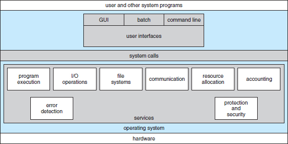
Figure 2.1 A view of operating system services.
One set of operating system services provides functions that are helpful to the user.
- User interface. Almost all operating systems have a user interface (UI). This interface can take several forms. One is a command-line interface (CLI), which uses text commands and a method for entering them (say, a keyboard for typing in commands in a specific format with specific options). Another is a batch interface, in which commands and directives to control those commands are entered into files, and those files are executed. Most commonly, a graphical user interface (GUI) is used. Here, the interface is a window system with a pointing device to direct I/O, choose from menus, and make selections and a keyboard to enter text. Some systems provide two or all three of these variations.
- Program execution. The system must be able to load a program into memory and to run that program. The program must be able to end its execution, either normally or abnormally (indicating error).
- I/O operations. A running program may require I/O, which may involve a file or an I/O device. For specific devices, special functions may be desired (such as recording to a CD or DVD drive or blanking a display screen). For efficiency and protection, users usually cannot control I/O devices directly. Therefore, the operating system must provide a means to do I/O.
- File-system manipulation. The file system is of particular interest. Obviously, programs need to read and write files and directories. They also need to create and delete them by name, search for a given file, and list file information. Finally, some operating systems include permissions management to allow or deny access to files or directories based on file ownership. Many operating systems provide a variety of file systems, sometimes to allow personal choice and sometimes to provide specific features or performance characteristics.
- Communications. There are many circumstances in which one process needs to exchange information with another process. Such communication may occur between processes that are executing on the same computer or between processes that are executing on different computer systems tied together by a computer network. Communications may be implemented via shared memory, in which two or more processes read and write to a shared section of memory, or message passing, in which packets of information in predefined formats are moved between processes by the operating system.
- Error detection. The operating system needs to be detecting and correcting errors constantly. Errors may occur in the CPU and memory hardware (such as a memory error or a power failure), in I/O devices (such as a parity error on disk, a connection failure on a network, or lack of paper in the printer), and in the user program (such as an arithmetic overflow, an attempt to access an illegal memory location, or a too-great use of CPU time). For each type of error, the operating system should take the appropriate action to ensure correct and consistent computing. Sometimes, it has no choice but to halt the system. At other times, it might terminate an error-causing process or return an error code to a process for the process to detect and possibly correct.
Another set of operating system functions exists not for helping the user but rather for ensuring the efficient operation of the system itself. Systems with multiple users can gain efficiency by sharing the computer resources among the users.
- Resource allocation. When there are multiple users or multiple jobs running at the same time, resources must be allocated to each of them. The operating system manages many different types of resources. Some (such as CPU cycles, main memory, and file storage) may have special allocation code, whereas others (such as I/O devices) may have much more general request and release code. For instance, in determining how best to use the CPU, operating systems have CPU-scheduling routines that take into account the speed of the CPU, the jobs that must be executed, the number of registers available, and other factors. There may also be routines to allocate printers, USB storage drives, and other peripheral devices.
- Accounting. We want to keep track of which users use how much and what kinds of computer resources. This record keeping may be used for accounting (so that users can be billed) or simply for accumulating usage statistics. Usage statistics may be a valuable tool for researchers who wish to reconfigure the system to improve computing services.
- Protection and security. The owners of information stored in a multiuser or networked computer system may want to control use of that information. When several separate processes execute concurrently, it should not be possible for one process to interfere with the others or with the operating system itself. Protection involves ensuring that all access to system resources is controlled. Security of the system from outsiders is also important. Such security starts with requiring each user to authenticate himself or herself to the system, usually by means of a password, to gain access to system resources. It extends to defending external I/O devices, including network adapters, from invalid access attempts and to recording all such connections for detection of break-ins. If a system is to be protected and secure, precautions must be instituted throughout it. A chain is only as strong as its weakest link.
2.2 User and Operating-System Interface
We mentioned earlier that there are several ways for users to interface with the operating system. Here, we discuss two fundamental approaches. One provides a command-line interface, or command interpreter, that allows users to directly enter commands to be performed by the operating system. The other allows users to interface with the operating system via a graphical user interface, or GUI.
2.2.1 Command Interpreters
Some operating systems include the command interpreter in the kernel. Others, such as Windows and UNIX, treat the command interpreter as a special program that is running when a job is initiated or when a user first logs on (on interactive systems). On systems with multiple command interpreters to choose from, the interpreters are known as shells. For example, on UNIX and Linux systems, a user may choose among several different shells, including the Bourne shell, C shell, Bourne-Again shell, Korn shell, and others. Third-party shells and free user-written shells are also available. Most shells provide similar functionality, and a user's choice of which shell to use is generally based on personal preference. Figure 2.2 shows the Bourne shell command interpreter being used on Solaris 10.
The main function of the command interpreter is to get and execute the next user-specified command. Many of the commands given at this level manipulate files: create, delete, list, print, copy, execute, and so on. The MS-DOS and UNIX shells operate in this way. These commands can be implemented in two general ways.
In one approach, the command interpreter itself contains the code to execute the command. For example, a command to delete a file may cause the command interpreter to jump to a section of its code that sets up the parameters and makes the appropriate system call. In this case, the number of commands that can be given determines the size of the command interpreter, since each command requires its own implementing code.
An alternative approach—used by UNIX, among other operating systems—implements most commands through system programs. In this case, the command interpreter does not understand the command in any way; it merely uses the command to identify a file to be loaded into memory and executed. Thus, the UNIX command to delete a file
rm file.txt
would search for a file called rm, load the file into memory, and execute it with the parameter file.txt. The function associated with the rm command would be defined completely by the code in the file rm. In this way, programmers can add new commands to the system easily by creating new files with the proper names. The command-interpreter program, which can be small, does not have to be changed for new commands to be added.
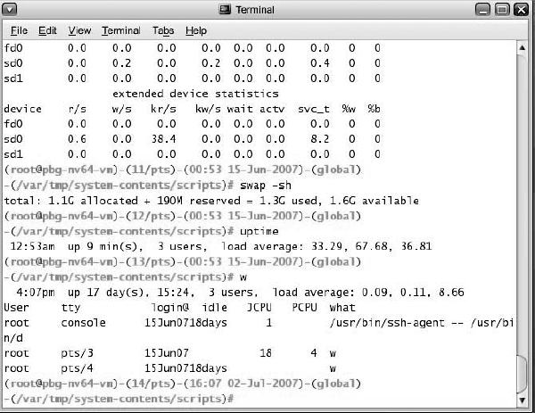
Figure 2.2 The Bourne shell command interpreter in Solrais 10.
2.2.2 Graphical User Interfaces
A second strategy for interfacing with the operating system is through a user-friendly graphical user interface, or GUI. Here, rather than entering commands directly via a command-line interface, users employ a mouse-based window-and-menu system characterized by a desktop metaphor. The user moves the mouse to position its pointer on images, or icons, on the screen (the desktop) that represent programs, files, directories, and system functions. Depending on the mouse pointer's location, clicking a button on the mouse can invoke a program, select a file or directory—known as a folder—or pull down a menu that contains commands.
Graphical user interfaces first appeared due in part to research taking place in the early 1970s at Xerox PARC research facility. The first GUI appeared on the Xerox Alto computer in 1973. However, graphical interfaces became more widespread with the advent of Apple Macintosh computers in the 1980s. The user interface for the Macintosh operating system (Mac OS) has undergone various changes over the years, the most significant being the adoption of the Aqua interface that appeared with Mac OS X. Microsoft's first version of Windows—Version 1.0—was based on the addition of a GUI interface to the MS-DOS operating system. Later versions of Windows have made cosmetic changes in the appearance of the GUI along with several enhancements in its functionality.
Because a mouse is impractical for most mobile systems, smartphones and handheld tablet computers typically use a touchscreen interface. Here, users interact by making gestures on the touchscreen—for example, pressing and swiping fingers across the screen. Figure 2.3 illustrates the touchscreen of the Apple iPad. Whereas earlier smartphones included a physical keyboard, most smartphones now simulate a keyboard on the touchscreen.
Traditionally, UNIX systems have been dominated by command-line interfaces. Various GUI interfaces are available, however. These include the Common Desktop Environment (CDE) and X-Windows systems, which are common on commercial versions of UNIX, such as Solaris and IBM's AIX system. In addition, there has been significant development in GUI designs from various open-source projects, such as K Desktop Environment (or KDE) and the GNOME desktop by the GNU project. Both the KDE and GNOME desktops run on Linux and various UNIX systems and are available under open-source licenses, which means their source code is readily available for reading and for modification under specific license terms.

Figure 2.3 The iPad touchscreen.
2.2.3 Choice of Interface
The choice of whether to use a command-line or GUI interface is mostly one of personal preference. System administrators who manage computers and power users who have deep knowledge of a system frequently use the command-line interface. For them, it is more efficient, giving them faster access to the activities they need to perform. Indeed, on some systems, only a subset of system functions is available via the GUI, leaving the less common tasks to those who are command-line knowledgeable. Further, command-line interfaces usually make repetitive tasks easier, in part because they have their own programmability. For example, if a frequent task requires a set of command-line steps, those steps can be recorded into a file, and that file can be run just like a program. The program is not compiled into executable code but rather is interpreted by the command-line interface. These shell scripts are very common on systems that are command-line oriented, such as UNIX and Linux.
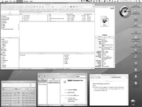
In contrast, most Windows users are happy to use the Windows GUI environment and almost never use the MS-DOS shell interface. The various changes undergone by the Macintosh operating systems provide a nice study in contrast. Historically, Mac OS has not provided a command-line interface, always requiring its users to interface with the operating system using its GUI. However, with the release of Mac OS X (which is in part implemented using a UNIX kernel), the operating system now provides both a Aqua interface and a command-line interface. Figure 2.4 is a screenshot of the Mac OS X GUI.
The user interface can vary from system to system and even from user to user within a system. It typically is substantially removed from the actual system structure. The design of a useful and friendly user interface is therefore not a direct function of the operating system. In this book, we concentrate on the fundamental problems of providing adequate service to user programs. From the point of view of the operating system, we do not distinguish between user programs and system programs.
2.3 System Calls
System calls provide an interface to the services made available by an operating system. These calls are generally available as routines written in C and C++, although certain low-level tasks (for example, tasks where hardware must be accessed directly) may have to be written using assembly-language instructions.
Before we discuss how an operating system makes system calls available, let's first use an example to illustrate how system calls are used: writing a simple program to read data from one file and copy them to another file. The first input that the program will need is the names of the two files: the input file and the output file. These names can be specified in many ways, depending on the operating-system design. One approach is for the program to ask the user for the names. In an interactive system, this approach will require a sequence of system calls, first to write a prompting message on the screen and then to read from the keyboard the characters that define the two files. On mouse-based and icon-based systems, a menu of file names is usually displayed in a window. The user can then use the mouse to select the source name, and a window can be opened for the destination name to be specified. This sequence requires many I/O system calls.
Once the two file names have been obtained, the program must open the input file and create the output file. Each of these operations requires another system call. Possible error conditions for each operation can require additional system calls. When the program tries to open the input file, for example, it may find that there is no file of that name or that the file is protected against access. In these cases, the program should print a message on the console (another sequence of system calls) and then terminate abnormally (another system call). If the input file exists, then we must create a new output file. We may find that there is already an output file with the same name. This situation may cause the program to abort (a system call), or we may delete the existing file (another system call) and create a new one (yet another system call). Another option, in an interactive system, is to ask the user (via a sequence of system calls to output the prompting message and to read the response from the terminal) whether to replace the existing file or to abort the program.
When both files are set up, we enter a loop that reads from the input file (a system call) and writes to the output file (another system call). Each read and write must return status information regarding various possible error conditions. On input, the program may find that the end of the file has been reached or that there was a hardware failure in the read (such as a parity error). The write operation may encounter various errors, depending on the output device (for example, no more disk space).
Finally, after the entire file is copied, the program may close both files (another system call), write a message to the console or window (more system calls), and finally terminate normally (the final system call). This system-call sequence is shown in Figure 2.5.
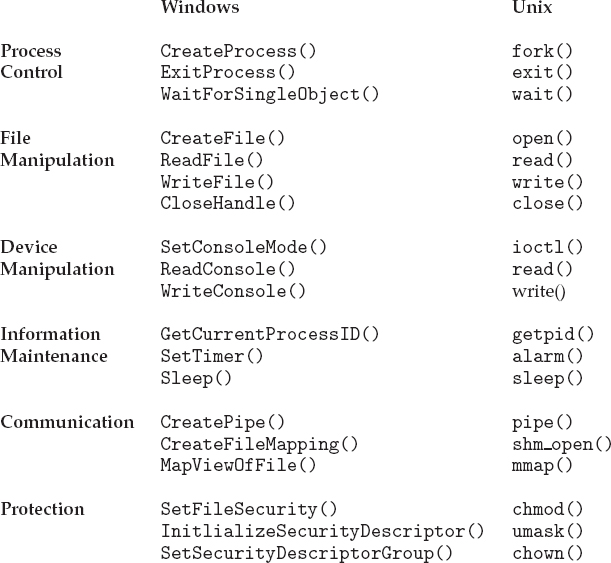
As you can see, even simple programs may make heavy use of the operating system. Frequently, systems execute thousands of system calls per second. Most programmers never see this level of detail, however. Typically, application developers design programs according to an application programming interface (API). The API specifies a set of functions that are available to an application programmer, including the parameters that are passed to each function and the return values the programmer can expect. Three of the most common APIs available to application programmers are the Windows API for Windows systems, the POSIX API for POSIX-based systems (which include virtually all versions of UNIX, Linux, and Mac OSX), and the Java API for programs that run on the Java virtual machine. A programmer accesses an API via a library of code provided by the operating system. In the case of UNIX and Linux for programs written in the C language, the library is called libc. Note that—unless specified—the system-call names used throughout this text are generic examples. Each operating system has its own name for each system call.
Behind the scenes, the functions that make up an API typically invoke the actual system calls on behalf of the application programmer. For example, the Windows function CreateProcess() (which unsurprisingly is used to create a new process) actually invokes the NTCreateProcess() system call in the Windows kernel.
Why would an application programmer prefer programming according to an API rather than invoking actual system calls? There are several reasons for doing so. One benefit concerns program portability. An application programmer designing a program using an API can expect her program to compile and run on any system that supports the same API (although, in reality, architectural differences often make this more difficult than it may appear). Furthermore, actual system calls can often be more detailed and difficult to work with than the API available to an application programmer. Nevertheless, there often exists a strong correlation between a function in the API and its associated system call within the kernel. In fact, many of the POSIX and Windows APIs are similar to the native system calls provided by the UNIX, Linux, and Windows operating systems.
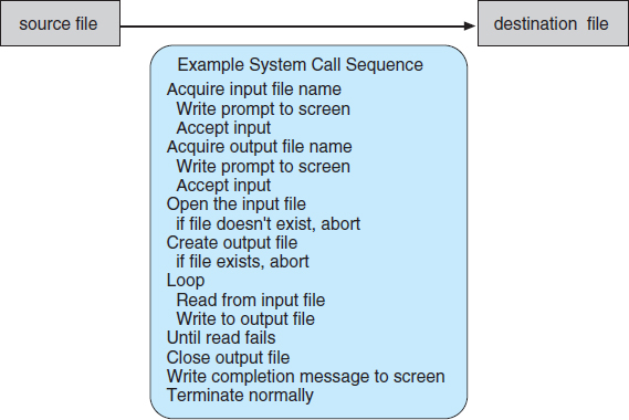
Figure 2.5 Example of how system calls are used.
EXAMPLE OF STANDARD API
As an example of a standard API, consider the read() function that is available in UNIX and Linux systems. The API for this function is obtained from the man page by invoking the command
man read
on the command line. A description of this API appears below:
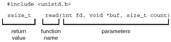
A program that uses the read() function must include the unistd.h header file, as this file defines the ssize_t and size_t data types (among other things). The parameters passed to read() are as follows:
- int fd—the file descriptor to be read
- void *buf—a buffer where the data will be read into
- size_t count—the maximum number of bytes to be read into the buffer
On a successful read, the number of bytes read is returned. A return value of 0 indicates end of file. If an error occurs, read() returns −1.
For most programming languages, the run-time support system (a set of functions built into libraries included with a compiler) provides a system-call interface that serves as the link to system calls made available by the operating system. The system-call interface intercepts function calls in the API and invokes the necessary system calls within the operating system. Typically, a number is associated with each system call, and the system-call interface maintains a table indexed according to these numbers. The system call interface then invokes the intended system call in the operating-system kernel and returns the status of the system call and any return values.
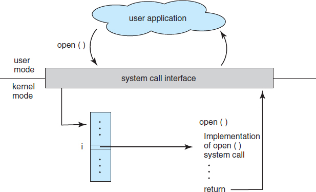
Figure 2.6 The handling of a user application invoking the open() system call.
The caller need know nothing about how the system call is implemented or what it does during execution. Rather, the caller need only obey the API and understand what the operating system will do as a result of the execution of that system call. Thus, most of the details of the operating-system interface are hidden from the programmer by the API and are managed by the run-time support library. The relationship between an API, the system-call interface, and the operating system is shown in Figure 2.6, which illustrates how the operating system handles a user application invoking the open() system call.
System calls occur in different ways, depending on the computer in use. Often, more information is required than simply the identity of the desired system call. The exact type and amount of information vary according to the particular operating system and call. For example, to get input, we may need to specify the file or device to use as the source, as well as the address and length of the memory buffer into which the input should be read. Of course, the device or file and length may be implicit in the call.
Three general methods are used to pass parameters to the operating system. The simplest approach is to pass the parameters in registers. In some cases, however, there may be more parameters than registers. In these cases, the parameters are generally stored in a block, or table, in memory, and the address of the block is passed as a parameter in a register (Figure 2.7). This is the approach taken by Linux and Solaris. Parameters also can be placed, or pushed, onto the stack by the program and popped off the stack by the operating system. Some operating systems prefer the block or stack method because those approaches do not limit the number or length of parameters being passed.
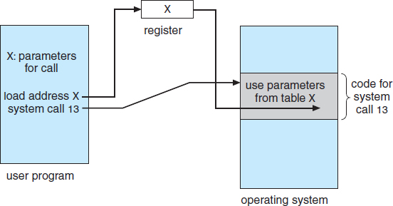
Figure 2.7 Passing of parameters as a table.
2.4 Types of System Calls
System calls can be grouped roughly into six major categories: process control, file manipulation, device manipulation, information maintenance, communications, and protection. In Sections 2.4.1 through 2.4.6, we briefly discuss the types of system calls that may be provided by an operating system. Most of these system calls support, or are supported by, concepts and functions that are discussed in later chapters. Figure 2.8 summarizes the types of system calls normally provided by an operating system. As mentioned, in this text, we normally refer to the system calls by generic names. Throughout the text, however, we provide examples of the actual counterparts to the system calls for Windows, UNIX, and Linux systems.
2.4.1 Process Control
A running program needs to be able to halt its execution either normally (end()) or abnormally (abort()). If a system call is made to terminate the currently running program abnormally, or if the program runs into a problem and causes an error trap, a dump of memory is sometimes taken and an error message generated. The dump is written to disk and may be examined by a debugger—a system program designed to aid the programmer in finding and correcting errors, or bugs—to determine the cause of the problem. Under either normal or abnormal circumstances, the operating system must transfer control to the invoking command interpreter. The command interpreter then reads the next command. In an interactive system, the command interpreter simply continues with the next command; it is assumed that the user will issue an appropriate command to respond to any error. In a GUI system, a pop-up window might alert the user to the error and ask for guidance. In a batch system, the command interpreter usually terminates the entire job and continues with the next job. Some systems may allow for special recovery actions in case an error occurs. If the program discovers an error in its input and wants to terminate abnormally, it may also want to define an error level. More severe errors can be indicated by a higher-level error parameter. It is then possible to combine normal and abnormal termination by defining a normal termination as an error at level 0. The command interpreter or a following program can use this error level to determine the next action automatically.
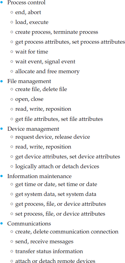
Figure 2.8 Types of system calls.
A process or job executing one program may want to load() and execute() another program. This feature allows the command interpreter to execute a program as directed by, for example, a user command, the click of a mouse, or a batch command. An interesting question is where to return control when the loaded program terminates. This question is related to whether the existing program is lost, saved, or allowed to continue execution concurrently with the new program.
EXAMPLES OF WINDOWS AND UNIX SYSTEM CALLS
If control returns to the existing program when the new program terminates, we must save the memory image of the existing program; thus, we have effectively created a mechanism for one program to call another program. If both programs continue concurrently, we have created a new job or process to be multiprogrammed. Often, there is a system call specifically for this purpose (create_process() or submit_job()).
If we create a new job or process, or perhaps even a set of jobs or processes, we should be able to control its execution. This control requires the ability to determine and reset the attributes of a job or process, including the job's priority, its maximum allowable execution time, and so on (get_process_attributes() and set_process_attributes()). We may also want to terminate a job or process that we created (terminate_process()) if we find that it is incorrect or is no longer needed.
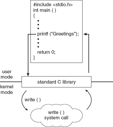
The standard C library provides a portion of the system-call interface for many versions of UNIX and Linux. As an example, let's assume a C program invokes the printf() statement. The C library intercepts this call and invokes the necessary system call (or calls) in the operating system—in this instance, the write() system call. The C library takes the value returned by write() and passes it back to the user program. This is shown below:
Having created new jobs or processes, we may need to wait for them to finish their execution. We may want to wait for a certain amount of time to pass (wait_time()). More probably, we will want to wait for a specific event to occur (wait_event()). The jobs or processes should then signal when that event has occurred (signal_event()).
Quite often, two or more processes may share data. To ensure the integrity of the data being shared, operating systems often provide system calls allowing a process to lock shared data. Then, no other process can access the data until the lock is released. Typically, such system calls include acquire_lock() and release_lock(). System calls of these types, dealing with the coordination of concurrent processes, are discussed in great detail in Chapter 5.
There are so many facets of and variations in process and job control that we next use two examples—one involving a single-tasking system and the other a multitasking system—to clarify these concepts. The MS-DOS operating system is an example of a single-tasking system. It has a command interpreter that is invoked when the computer is started (Figure 2.9(a)). Because MS-DOS is single-tasking, it uses a simple method to run a program and does not create a new process. It loads the program into memory, writing over most of itself to give the program as much memory as possible (Figure 2.9(b)). Next, it sets the instruction pointer to the first instruction of the program. The program then runs, and either an error causes a trap, or the program executes a system call to terminate. In either case, the error code is saved in the system memory for later use. Following this action, the small portion of the command interpreter that was not overwritten resumes execution. Its first task is to reload the rest of the command interpreter from disk. Then the command interpreter makes the previous error code available to the user or to the next program.
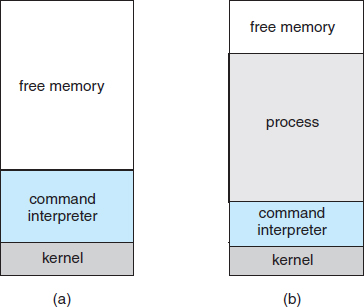
Figure 2.9 MS-DOS execution. (a) At system startup. (b) Running a program.
FreeBSD (derived from Berkeley UNIX) is an example of a multitasking system. When a user logs on to the system, the shell of the user's choice is run. This shell is similar to the MS-DOS shell in that it accepts commands and executes programs that the user requests. However, since FreeBSD is a multitasking system, the command interpreter may continue running while another program is executed (Figure 2.10). To start a new process, the shell executes a fork() system call. Then, the selected program is loaded into memory via an exec() system call, and the program is executed. Depending on the way the command was issued, the shell then either waits for the process to finish or runs the process “in the background.” In the latter case, the shell immediately requests another command. When a process is running in the background, it cannot receive input directly from the keyboard, because the shell is using this resource. I/O is therefore done through files or through a GUI interface. Meanwhile, the user is free to ask the shell to run other programs, to monitor the progress of the running process, to change that program's priority, and so on. When the process is done, it executes an exit() system call to terminate, returning to the invoking process a status code of 0 or a nonzero error code. This status or error code is then available to the shell or other programs. Processes are discussed in Chapter 3 with a program example using the fork() and exec() system calls.
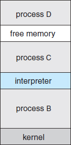
Figure 2.10 FreeBSD running multiple programs.
2.4.2 File Management
The file system is discussed in more detail in Chapters 11 and 12. We can, however, identify several common system calls dealing with files.
We first need to be able to create() and delete() files. Either system call requires the name of the file and perhaps some of the file's attributes. Once the file is created, we need to open() it and to use it. We may also read(), write(), or reposition() (rewind or skip to the end of the file, for example). Finally, we need to close() the file, indicating that we are no longer using it.
We may need these same sets of operations for directories if we have a directory structure for organizing files in the file system. In addition, for either files or directories, we need to be able to determine the values of various attributes and perhaps to reset them if necessary. File attributes include the file name, file type, protection codes, accounting information, and so on. At least two system calls, get_file_attributes() and set_file_attributes(), are required for this function. Some operating systems provide many more calls, such as calls for file move() and copy(). Others might provide an API that performs those operations using code and other system calls, and others might provide system programs to perform those tasks. If the system programs are callable by other programs, then each can be considered an API by other system programs.
2.4.3 Device Management
A process may need several resources to execute—main memory, disk drives, access to files, and so on. If the resources are available, they can be granted, and control can be returned to the user process. Otherwise, the process will have to wait until sufficient resources are available.
The various resources controlled by the operating system can be thought of as devices. Some of these devices are physical devices (for example, disk drives), while others can be thought of as abstract or virtual devices (for example, files). A system with multiple users may require us to first request() a device, to ensure exclusive use of it. After we are finished with the device, we release() it. These functions are similar to the open() and close() system calls for files. Other operating systems allow unmanaged access to devices. The hazard then is the potential for device contention and perhaps deadlock, which are described in Chapter 7.
Once the device has been requested (and allocated to us), we can read(), write(), and (possibly) reposition() the device, just as we can with files. In fact, the similarity between I/O devices and files is so great that many operating systems, including UNIX, merge the two into a combined file–device structure. In this case, a set of system calls is used on both files and devices. Sometimes, I/O devices are identified by special file names, directory placement, or file attributes.
The user interface can also make files and devices appear to be similar, even though the underlying system calls are dissimilar. This is another example of the many design decisions that go into building an operating system and user interface.
2.4.4 Information Maintenance
Many system calls exist simply for the purpose of transferring information between the user program and the operating system. For example, most systems have a system call to return the current time() and date(). Other system calls may return information about the system, such as the number of current users, the version number of the operating system, the amount of free memory or disk space, and so on.
Another set of system calls is helpful in debugging a program. Many systems provide system calls to dump() memory. This provision is useful for debugging. A program trace lists each system call as it is executed. Even microprocessors provide a CPU mode known as single step, in which a trap is executed by the CPU after every instruction. The trap is usually caught by a debugger.
Many operating systems provide a time profile of a program to indicate the amount of time that the program executes at a particular location or set of locations. A time profile requires either a tracing facility or regular timer interrupts. At every occurrence of the timer interrupt, the value of the program counter is recorded. With sufficiently frequent timer interrupts, a statistical picture of the time spent on various parts of the program can be obtained.
In addition, the operating system keeps information about all its processes, and system calls are used to access this information. Generally, calls are also used to reset the process information (get_process_attributes() and set_process_attributes()). In Section 3.1.3, we discuss what information is normally kept.
2.4.5 Communication
There are two common models of interprocess communication: the message-passing model and the shared-memory model. In the message-passing model, the communicating processes exchange messages with one another to transfer information. Messages can be exchanged between the processes either directly or indirectly through a common mailbox. Before communication can take place, a connection must be opened. The name of the other communicator must be known, be it another process on the same system or a process on another computer connected by a communications network. Each computer in a network has a host name by which it is commonly known. A host also has a network identifier, such as an IP address. Similarly, each process has a process name, and this name is translated into an identifier by which the operating system can refer to the process. The get_hostid() and get_processid() system calls do this translation. The identifiers are then passed to the general-purpose open() and close() calls provided by the file system or to specific open_connection() and close_connection() system calls, depending on the system's model of communication. The recipient process usually must give its permission for communication to take place with an accept_connection() call. Most processes that will be receiving connections are special-purpose daemons, which are system programs provided for that purpose. They execute a wait_for_connection() call and are awakened when a connection is made. The source of the communication, known as the client, and the receiving daemon, known as a server, then exchange messages by using read_message() and write_message() system calls. The close_connection() call terminates the communication.
In the shared-memory model, processes use shared_memory_create() and shared_memory_attach() system calls to create and gain access to regions of memory owned by other processes. Recall that, normally, the operating system tries to prevent one process from accessing another process's memory. Shared memory requires that two or more processes agree to remove this restriction. They can then exchange information by reading and writing data in the shared areas. The form of the data is determined by the processes and is not under the operating system's control. The processes are also responsible for ensuring that they are not writing to the same location simultaneously. Such mechanisms are discussed in Chapter 5. In Chapter 4, we look at a variation of the process scheme—threads—in which memory is shared by default.
Both of the models just discussed are common in operating systems, and most systems implement both. Message passing is useful for exchanging smaller amounts of data, because no conflicts need be avoided. It is also easier to implement than is shared memory for intercomputer communication. Shared memory allows maximum speed and convenience of communication, since it can be done at memory transfer speeds when it takes place within a computer. Problems exist, however, in the areas of protection and synchronization between the processes sharing memory.
2.4.6 Protection
Protection provides a mechanism for controlling access to the resources provided by a computer system. Historically, protection was a concern only on multiprogrammed computer systems with several users. However, with the advent of networking and the Internet, all computer systems, from servers to mobile handheld devices, must be concerned with protection.
Typically, system calls providing protection include set_permission() and get_permission(), which manipulate the permission settings of resources such as files and disks. The allow_user() and deny_user() system calls specify whether particular users can—or cannot—be allowed access to certain resources.
We cover protection in Chapter 14 and the much larger issue of security in Chapter 15.
2.5 System Programs
Another aspect of a modern system is its collection of system programs. Recall Figure 1.1, which depicted the logical computer hierarchy. At the lowest level is hardware. Next is the operating system, then the system programs, and finally the application programs. System programs, also known as system utilities, provide a convenient environment for program development and execution. Some of them are simply user interfaces to system calls. Others are considerably more complex. They can be divided into these categories:
- File management. These programs create, delete, copy, rename, print, dump, list, and generally manipulate files and directories.
- Status information. Some programs simply ask the system for the date, time, amount of available memory or disk space, number of users, or similar status information. Others are more complex, providing detailed performance, logging, and debugging information. Typically, these programs format and print the output to the terminal or other output devices or files or display it in a window of the GUI. Some systems also support a registry, which is used to store and retrieve configuration information.
- File modification. Several text editors may be available to create and modify the content of files stored on disk or other storage devices. There may also be special commands to search contents of files or perform transformations of the text.
- Programming-language support. Compilers, assemblers, debuggers, and interpreters for common programming languages (such as C, C++, Java, and PERL) are often provided with the operating system or available as a separate download.
- Program loading and execution. Once a program is assembled or compiled, it must be loaded into memory to be executed. The system may provide absolute loaders, relocatable loaders, linkage editors, and overlay loaders. Debugging systems for either higher-level languages or machine language are needed as well.
- Communications. These programs provide the mechanism for creating virtual connections among processes, users, and computer systems. They allow users to send messages to one another's screens, to browse Web pages, to send e-mail messages, to log in remotely, or to transfer files from one machine to another.
- Background services. All general-purpose systems have methods for launching certain system-program processes at boot time. Some of these processes terminate after completing their tasks, while others continue to run until the system is halted. Constantly running system-program processes are known as services, subsystems, or daemons. One example is the network daemon discussed in Section 2.4.5. In that example, a system needed a service to listen for network connections in order to connect those requests to the correct processes. Other examples include process schedulers that start processes according to a specified schedule, system error monitoring services, and print servers. Typical systems have dozens of daemons. In addition, operating systems that run important activities in user context rather than in kernel context may use daemons to run these activities.
Along with system programs, most operating systems are supplied with programs that are useful in solving common problems or performing common operations. Such application programs include Web browsers, word processors and text formatters, spreadsheets, database systems, compilers, plotting and statistical-analysis packages, and games.
The view of the operating system seen by most users is defined by the application and system programs, rather than by the actual system calls. Consider a user's PC. When a user's computer is running the Mac OS X operating system, the user might see the GUI, featuring a mouse-and-windows interface. Alternatively, or even in one of the windows, the user might have a command-line UNIX shell. Both use the same set of system calls, but the system calls look different and act in different ways. Further confusing the user view, consider the user dual-booting from Mac OS X into Windows. Now the same user on the same hardware has two entirely different interfaces and two sets of applications using the same physical resources. On the same hardware, then, a user can be exposed to multiple user interfaces sequentially or concurrently.
2.6 Operating-System Design and Implementation
In this section, we discuss problems we face in designing and implementing an operating system. There are, of course, no complete solutions to such problems, but there are approaches that have proved successful.
2.6.1 Design Goals
The first problem in designing a system is to define goals and specifications. At the highest level, the design of the system will be affected by the choice of hardware and the type of system: batch, time sharing, single user, multiuser, distributed, real time, or general purpose.
Beyond this highest design level, the requirements may be much harder to specify. The requirements can, however, be divided into two basic groups: user goals and system goals.
Users want certain obvious properties in a system. The system should be convenient to use, easy to learn and to use, reliable, safe, and fast. Of course, these specifications are not particularly useful in the system design, since there is no general agreement on how to achieve them.
A similar set of requirements can be defined by those people who must design, create, maintain, and operate the system. The system should be easy to design, implement, and maintain; and it should be flexible, reliable, error free, and efficient. Again, these requirements are vague and may be interpreted in various ways.
There is, in short, no unique solution to the problem of defining the requirements for an operating system. The wide range of systems in existence shows that different requirements can result in a large variety of solutions for different environments. For example, the requirements for VxWorks, a real-time operating system for embedded systems, must have been substantially different from those for MVS, a large multiuser, multiaccess operating system for IBM mainframes.
Specifying and designing an operating system is a highly creative task. Although no textbook can tell you how to do it, general principles have been developed in the field of software engineering, and we turn now to a discussion of some of these principles.
2.6.2 Mechanisms and Policies
One important principle is the separation of policy from mechanism. Mechanisms determine how to do something; policies determine what will be done. For example, the timer construct (see Section 1.5.2) is a mechanism for ensuring CPU protection, but deciding how long the timer is to be set for a particular user is a policy decision.
The separation of policy and mechanism is important for flexibility. Policies are likely to change across places or over time. In the worst case, each change in policy would require a change in the underlying mechanism. A general mechanism insensitive to changes in policy would be more desirable. A change in policy would then require redefinition of only certain parameters of the system. For instance, consider a mechanism for giving priority to certain types of programs over others. If the mechanism is properly separated from policy, it can be used either to support a policy decision that I/O-intensive programs should have priority over CPU-intensive ones or to support the opposite policy.
Microkernel-based operating systems (Section 2.7.3) take the separation of mechanism and policy to one extreme by implementing a basic set of primitive building blocks. These blocks are almost policy free, allowing more advanced mechanisms and policies to be added via user-created kernel modules or user programs themselves. As an example, consider the history of UNIX. At first, it had a time-sharing scheduler. In the latest version of Solaris, scheduling is controlled by loadable tables. Depending on the table currently loaded, the system can be time sharing, batch processing, real time, fair share, or any combination. Making the scheduling mechanism general purpose allows vast policy changes to be made with a single load-new-table command. At the other extreme is a system such as Windows, in which both mechanism and policy are encoded in the system to enforce a global look and feel. All applications have similar interfaces, because the interface itself is built into the kernel and system libraries. The Mac OS X operating system has similar functionality.
Policy decisions are important for all resource allocation. Whenever it is necessary to decide whether or not to allocate a resource, a policy decision must be made. Whenever the question is how rather than what, it is a mechanism that must be determined.
2.6.3 Implementation
Once an operating system is designed, it must be implemented. Because operating systems are collections of many programs, written by many people over a long period of time, it is difficult to make general statements about how they are implemented.
Early operating systems were written in assembly language. Now, although some operating systems are still written in assembly language, most are written in a higher-level language such as C or an even higher-level language such as C++. Actually, an operating system can be written in more than one language. The lowest levels of the kernel might be assembly language. Higher-level routines might be in C, and system programs might be in C or C++, in interpreted scripting languages like PERL or Python, or in shell scripts. In fact, a given Linux distribution probably includes programs written in all of those languages.
The first system that was not written in assembly language was probably the Master Control Program (MCP) for Burroughs computers. MCP was written in a variant of ALGOL. MULTICS, developed at MIT, was written mainly in the system programming language PL/1. The Linux and Windows operating system kernels are written mostly in C, although there are some small sections of assembly code for device drivers and for saving and restoring the state of registers.
The advantages of using a higher-level language, or at least a systems-implementation language, for implementing operating systems are the same as those gained when the language is used for application programs: the code can be written faster, is more compact, and is easier to understand and debug. In addition, improvements in compiler technology will improve the generated code for the entire operating system by simple recompilation. Finally, an operating system is far easier to port—to move to some other hardware—if it is written in a higher-level language. For example, MS-DOS was written in Intel 8088 assembly language. Consequently, it runs natively only on the Intel X86 family of CPUs. (Note that although MS-DOS runs natively only on Intel X86, emulators of the X86 instruction set allow the operating system to run on other CPUs—but more slowly, and with higher resource use. As we mentioned in Chapter 1, emulators are programs that duplicate the functionality of one system on another system.) The Linux operating system, in contrast, is written mostly in C and is available natively on a number of different CPUs, including Intel X86, Oracle SPARC, and IBMPowerPC.
The only possible disadvantages of implementing an operating system in a higher-level language are reduced speed and increased storage requirements. This, however, is no longer a major issue in today's systems. Although an expert assembly-language programmer can produce efficient small routines, for large programs a modern compiler can perform complex analysis and apply sophisticated optimizations that produce excellent code. Modern processors have deep pipelining and multiple functional units that can handle the details of complex dependencies much more easily than can the human mind.
As is true in other systems, major performance improvements in operating systems are more likely to be the result of better data structures and algorithms than of excellent assembly-language code. In addition, although operating systems are large, only a small amount of the code is critical to high performance; the interrupt handler, I/O manager, memory manager, and CPU scheduler are probably the most critical routines. After the system is written and is working correctly, bottleneck routines can be identified and can be replaced with assembly-language equivalents.
2.7 Operating-System Structure
A system as large and complex as a modern operating system must be engineered carefully if it is to function properly and be modified easily. A common approach is to partition the task into small components, or modules, rather than have one monolithic system. Each of these modules should be a well-defined portion of the system, with carefully defined inputs, outputs, and functions. We have already discussed briefly in Chapter 1 the common components of operating systems. In this section, we discuss how these components are interconnected and melded into a kernel.
2.7.1 Simple Structure
Many operating systems do not have well-defined structures. Frequently, such systems started as small, simple, and limited systems and then grew beyond their original scope. MS-DOS is an example of such a system. It was originally designed and implemented by a few people who had no idea that it would become so popular. It was written to provide the most functionality in the least space, so it was not carefully divided into modules. Figure 2.11 shows its structure.
In MS-DOS, the interfaces and levels of functionality are not well separated. For instance, application programs are able to access the basic I/O routines to write directly to the display and disk drives. Such freedom leaves MS-DOS vulnerable to errant (or malicious) programs, causing entire system crashes when user programs fail. Of course, MS-DOS was also limited by the hardware of its era. Because the Intel 8088 for which it was written provides no dual mode and no hardware protection, the designers of MS-DOS had no choice but to leave the base hardware accessible.
Another example of limited structuring is the original UNIX operating system. Like MS-DOS, UNIX initially was limited by hardware functionality. It consists of two separable parts: the kernel and the system programs. The kernel is further separated into a series of interfaces and device drivers, which have been added and expanded over the years as UNIX has evolved. We can view the traditional UNIX operating system as being layered to some extent, as shown in Figure 2.12. Everything below the system-call interface and above the physical hardware is the kernel. The kernel provides the file system, CPU scheduling, memory management, and other operating-system functions through system calls. Taken in sum, that is an enormous amount of functionality to be combined into one level. This monolithic structure was difficult to implement and maintain. It had a distinct performance advantage, however: there is very little overhead in the system call interface or in communication within the kernel. We still see evidence of this simple, monolithic structure in the UNIX, Linux, and Windows operating systems.
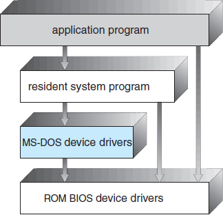
Figure 2.11 MS-DOS layer structure.
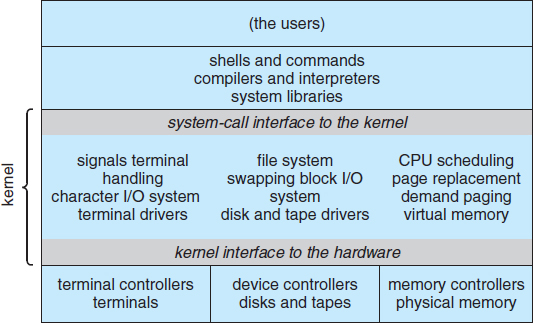
Figure 2.12 Traditional UNIX system structure.
2.7.2 Layered Approach
With proper hardware support, operating systems can be broken into pieces that are smaller and more appropriate than those allowed by the original MS-DOS and UNIX systems. The operating system can then retain much greater control over the computer and over the applications that make use of that computer. Implementers have more freedom in changing the inner workings of the system and in creating modular operating systems. Under a top-down approach, the overall functionality and features are determined and are separated into components. Information hiding is also important, because it leaves programmers free to implement the low-level routines as they see fit, provided that the external interface of the routine stays unchanged and that the routine itself performs the advertised task.
A system can be made modular in many ways. One method is the layered approach, in which the operating system is broken into a number of layers (levels). The bottom layer (layer 0) is the hardware; the highest (layer N) is the user interface. This layering structure is depicted in Figure 2.13.
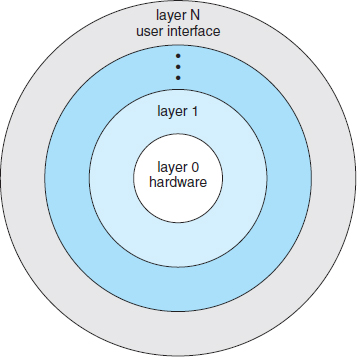
Figure 2.13 A layered operating system.
An operating-system layer is an implementation of an abstract object made up of data and the operations that can manipulate those data. A typical operating-system layer—say, layer M—consists of data structures and a set of routines that can be invoked by higher-level layers. Layer M, in turn, can invoke operations on lower-level layers.
The main advantage of the layered approach is simplicity of construction and debugging. The layers are selected so that each uses functions (operations) and services of only lower-level layers. This approach simplifies debugging and system verification. The first layer can be debugged without any concern for the rest of the system, because, by definition, it uses only the basic hardware (which is assumed correct) to implement its functions. Once the first layer is debugged, its correct functioning can be assumed while the second layer is debugged, and so on. If an error is found during the debugging of a particular layer, the error must be on that layer, because the layers below it are already debugged. Thus, the design and implementation of the system are simplified.
Each layer is implemented only with operations provided by lower-level layers. A layer does not need to know how these operations are implemented; it needs to know only what these operations do. Hence, each layer hides the existence of certain data structures, operations, and hardware from higher-level layers.
The major difficulty with the layered approach involves appropriately defining the various layers. Because a layer can use only lower-level layers, careful planning is necessary. For example, the device driver for the backing store (disk space used by virtual-memory algorithms) must be at a lower level than the memory-management routines, because memory management requires the ability to use the backing store.
Other requirements may not be so obvious. The backing-store driver would normally be above the CPU scheduler, because the driver may need to wait for I/O and the CPU can be rescheduled during this time. However, on a large system, the CPU scheduler may have more information about all the active processes than can fit in memory. Therefore, this information may need to be swapped in and out of memory, requiring the backing-store driver routine to be below the CPU scheduler.
A final problem with layered implementations is that they tend to be less efficient than other types. For instance, when a user program executes an I/O operation, it executes a system call that is trapped to the I/O layer, which calls the memory-management layer, which in turn calls the CPU-scheduling layer, which is then passed to the hardware. At each layer, the parameters may be modified, data may need to be passed, and so on. Each layer adds overhead to the system call. The net result is a system call that takes longer than does one on a nonlayered system.
These limitations have caused a small backlash against layering in recent years. Fewer layers with more functionality are being designed, providing most of the advantages of modularized code while avoiding the problems of layer definition and interaction.
2.7.3 Microkernels
We have already seen that as UNIX expanded, the kernel became large and difficult to manage. In the mid-1980s, researchers at Carnegie Mellon University developed an operating system called Mach that modularized the kernel using the microkernel approach. This method structures the operating system by removing all nonessential components from the kernel and implementing them as system and user-level programs. The result is a smaller kernel. There is little consensus regarding which services should remain in the kernel and which should be implemented in user space. Typically, however, microkernels provide minimal process and memory management, in addition to a communication facility. Figure 2.14 illustrates the architecture of a typical microkernel.
The main function of the microkernel is to provide communication between the client program and the various services that are also running in user space. Communication is provided through message passing, which was described in Section 2.4.5. For example, if the client program wishes to access a file, it must interact with the file server. The client program and service never interact directly. Rather, they communicate indirectly by exchanging messages with the microkernel.
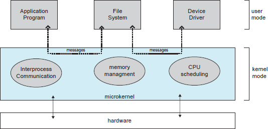
Figure 2.14 Architecture of a typical microkernel.
One benefit of the microkernel approach is that it makes extending the operating system easier. All new services are added to user space and consequently do not require modification of the kernel. When the kernel does have to be modified, the changes tend to be fewer, because the microkernel is a smaller kernel. The resulting operating system is easier to port from one hardware design to another. The microkernel also provides more security and reliability, since most services are running as user—rather than kernel—processes. If a service fails, the rest of the operating system remains untouched.
Some contemporary operating systems have used the microkernel approach. Tru64 UNIX(formerly Digital UNIX) provides a UNIX interface to the user, but it is implemented with a Mach kernel. The Mach kernel maps UNIX system calls into messages to the appropriate user-level services. The Mac OS X kernel (also known as Darwin) is also partly based on the Mach microkernel.
Another example is QNX, a real-time operating system for embedded systems. The QNX Neutrino microkernel provides services for message passing and process scheduling. It also handles low-level network communication and hardware interrupts. All other services in QNX are provided by standard processes that run outside the kernel in user mode.
Unfortunately, the performance of microkernels can suffer due to increased system-function overhead. Consider the history of Windows NT. The first release had a layered microkernel organization. This version's performance was low compared with that of Windows 95. Windows NT 4.0 partially corrected the performance problem by moving layers from user space to kernel space and integrating them more closely. By the time Windows XP was designed, Windows architecture had become more monolithic than microkernel.
2.7.4 Modules
Perhaps the best current methodology for operating-system design involves using loadable kernel modules. Here, the kernel has a set of core components and links in additional services via modules, either at boot time or during run time. This type of design is common in modern implementations of UNIX, such as Solaris, Linux, and Mac OS X, as well as Windows.
The idea of the design is for the kernel to provide core services while other services are implemented dynamically, as the kernel is running. Linking services dynamically is preferable to adding new features directly to the kernel, which would require recompiling the kernel every time a change was made. Thus, for example, we might build CPU scheduling and memory management algorithms directly into the kernel and then add support for different file systems by way of loadable modules.
The overall result resembles a layered system in that each kernel section has defined, protected interfaces; but it is more flexible than a layered system, because any module can call any other module. The approach is also similar to the microkernel approach in that the primary module has only core functions and knowledge of how to load and communicate with other modules; but it is more efficient, because modules do not need to invoke message passing in order to communicate.
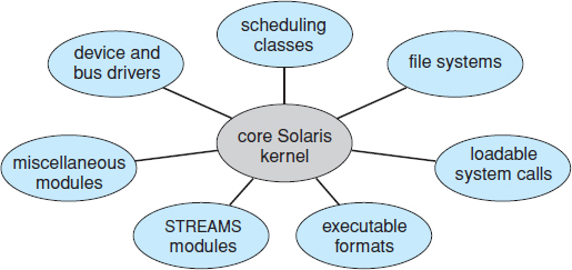
Figure 2.15 Solaris loadable modules.
The Solaris operating system structure, shown in Figure 2.15, is organized around a core kernel with seven types of loadable kernel modules:
- Scheduling classes
- File systems
- Loadable system calls
- Executable formats
- STREAMS modules
- Miscellaneous
- Device and bus drivers
Linux also uses loadable kernel modules, primarily for supporting device drivers and file systems. We cover creating loadable kernel modules in Linux as a programming exercise at the end of this chapter.
2.7.5 Hybrid Systems
In practice, very few operating systems adopt a single, strictly defined structure. Instead, they combine different structures, resulting in hybrid systems that address performance, security, and usability issues. For example, both Linux and Solaris are monolithic, because having the operating system in a single address space provides very efficient performance. However, they are also modular, so that new functionality can be dynamically added to the kernel. Windows is largely monolithic as well (again primarily for performance reasons), but it retains some behavior typical of microkernel systems, including providing support for separate subsystems (known as operating-system personalities) that run as user-mode processes. Windows systems also provide support for dynamically loadable kernel modules. We provide case studies of Linux and Windows 7 in in Chapters 18 and 19, respectively. In the remainder of this section, we explore the structure of three hybrid systems: the Apple Mac OS X operating system and the two most prominent mobile operating systems—iOS and Android.
2.7.5.1 Mac OS X
The Apple Mac OS X operating system uses a hybrid structure. As shown in Figure 2.16, it is a layered system. The top layers include the Aqua user interface (Figure 2.4) and a set of application environments and services. Notably, the Cocoa environment specifies an API for the Objective-C programming language, which is used for writing Mac OS X applications. Below these layers is the kernel environment, which consists primarily of the Mach microkernel and the BSD UNIX kernel. Mach provides memory management; support for remote procedure calls (RPCs) and interprocess communication (IPC) facilities, including message passing; and thread scheduling. The BSD component provides a BSD command-line interface, support for networking and file systems, and an implementation of POSIX APIs, including Pthreads. In addition to Mach and BSD, the kernel environment provides an I/O kit for development of device drivers and dynamically loadable modules (which Mac OS X refers to as kernel extensions). As shown in Figure 2.16, the BSD application environment can make use of BSD facilities directly.
2.7.5.2 iOS
iOS is a mobile operating system designed by Apple to run its smartphone, the iPhone, as well as its tablet computer, the iPad. iOS is structured on the Mac OS X operating system, with added functionality pertinent to mobile devices, but does not directly run Mac OS X applications. The structure of iOS appears in Figure 2.17.
Cocoa Touch is an API for Objective-C that provides several frameworks for developing applications that run on iOS devices. The fundamental difference between Cocoa, mentioned earlier, and Cocoa Touch is that the latter provides support for hardware features unique to mobile devices, such as touch screens. The media services layer provides services for graphics, audio, and video. The core services layer provides a variety of features, including support for cloud computing and databases. The bottom layer represents the core operating system, which is based on the kernel environment shown in Figure 2.16.
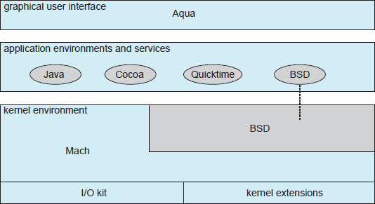
Figure 2.16 The Mac OS X structure.
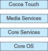
Figure 2.17 Architecture of Apple's iOS.
2.7.5.3 Android
The Android operating system was designed by the Open Handset Alliance (led primarily by Google) and was developed for Android smartphones and tablet computers. Whereas iOS is designed to run on Apple mobile devices and is close-sourced, Android runs on a variety of mobile platforms and is open-sourced, partly explaining its rapid rise in popularity. The structure of Android appears in Figure 2.18.
Android is similar to iOS in that it is a layered stack of software that provides a rich set of frameworks for developing mobile applications. At the bottom of this software stack is the Linux kernel, although it has been modified by Google and is currently outside the normal distribution of Linux releases. Linux is used primarily for process, memory, and device-driver support for hardware and has been expanded to include power management. The Android runtime environment includes a core set of libraries as well as the Dalvik virtual machine. Software designers for Android devices develop applications in the Java language. However, rather than using the standard Java API, Google has designed a separate Android API for Java development. The Java class files are first compiled to Java bytecode and then translated into an executable file that runs on the Dalvik virtual machine. The Dalvik virtual machine was designed for Android and is optimized for mobile devices with limited memory and CPU processing capabilities.
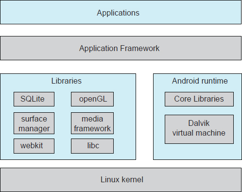
Figure 2.18 Architecture of Google's Android.
The set of libraries available for Android applications includes frameworks for developing web browsers (webkit), database support (SQLite), and multimedia. The libc library is similar to the standard C library but is much smaller and has been designed for the slower CPUs that characterize mobile devices.
2.8 Operating-System Debugging
We have mentioned debugging frequently in this chapter. Here, we take a closer look. Broadly, debugging is the activity of finding and fixing errors in a system, both in hardware and in software. Performance problems are considered bugs, so debugging can also include performance tuning, which seeks to improve performance by removing processing bottlenecks. In this section, we explore debugging process and kernel errors and performance problems. Hardware debugging is outside the scope of this text.
2.8.1 Failure Analysis
If a process fails, most operating systems write the error information to a log file to alert system operators or users that the problem occurred. The operating system can also take a core dump—a capture of the memory of the process—and store it in a file for later analysis. (Memory was referred to as the “core” in the early days of computing.) Running programs and core dumps can be probed by a debugger, which allows a programmer to explore the code and memory of a process.
Debugging user-level process code is a challenge. Operating-system kernel debugging is even more complex because of the size and complexity of the kernel, its control of the hardware, and the lack of user-level debugging tools. A failure in the kernel is called a crash. When a crash occurs, error information is saved to a log file, and the memory state is saved to a crash dump.
Operating-system debugging and process debugging frequently use different tools and techniques due to the very different nature of these two tasks. Consider that a kernel failure in the file-system code would make it risky for the kernel to try to save its state to a file on the file system before rebooting. A common technique is to save the kernel's memory state to a section of disk set aside for this purpose that contains no file system. If the kernel detects an unrecoverable error, it writes the entire contents of memory, or at least the kernel-owned parts of the system memory, to the disk area. When the system reboots, a process runs to gather the data from that area and write it to a crash dump file within a file system for analysis. Obviously, such strategies would be unnecessary for debugging ordinary user-level processes.
Kernighan's Law
“Debugging is twice as hard as writing the code in the first place. Therefore, if you write the code as cleverly as possible, you are, by definition, not smart enough to debug it.”
2.8.2 Performance Tuning
We mentioned earlier that performance tuning seeks to improve performance by removing processing bottlenecks. To identify bottlenecks, we must be able to monitor system performance. Thus, the operating system must have some means of computing and displaying measures of system behavior. In a number of systems, the operating system does this by producing trace listings of system behavior. All interesting events are logged with their time and important parameters and are written to a file. Later, an analysis program can process the log file to determine system performance and to identify bottlenecks and inefficiencies. These same traces can be run as input for a simulation of a suggested improved system. Traces also can help people to find errors in operating-system behavior.
Another approach to performance tuning uses single-purpose, interactive tools that allow users and administrators to question the state of various system components to look for bottlenecks. One such tool employs the UNIX command top to display the resources used on the system, as well as a sorted list of the “top” resource-using processes. Other tools display the state of disk I/O, memory allocation, and network traffic.
The Windows Task Manager is a similar tool for Windows systems. The task manager includes information for current applications as well as processes, CPU and memory usage, and networking statistics. A screen shot of the task manager appears in Figure 2.19.
Making operating systems easier to understand, debug, and tune as they run is an active area of research and implementation. A new generation of kernel-enabled performance analysis tools has made significant improvements in how this goal can be achieved. Next, we discuss a leading example of such a tool: the Solaris 10 DTrace dynamic tracing facility.
2.8.3 DTrace
DTrace is a facility that dynamically adds probes to a running system, both in user processes and in the kernel. These probes can be queried via the D programming language to determine an astonishing amount about the kernel, the system state, and process activities. For example, Figure 2.20 follows an application as it executes a system call (ioctl()) and shows the functional calls within the kernel as they execute to perform the system call. Lines ending with “U” are executed in user mode, and lines ending in “K” in kernel mode.
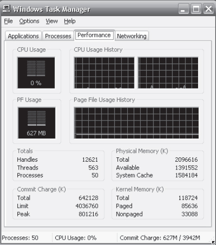
Figure 2.19 The Windows task manager.
Debugging the interactions between user-level and kernel code is nearly impossible without a toolset that understands both sets of code and can instrument the interactions. For that toolset to be truly useful, it must be able to debug any area of a system, including areas that were not written with debugging in mind, and do so without affecting system reliability. This tool must also have a minimum performance impact—ideally it should have no impact when not in use and a proportional impact during use. The DTrace tool meets these requirements and provides a dynamic, safe, low-impact debugging environment.
Until the DTrace framework and tools became available with Solaris 10, kernel debugging was usually shrouded in mystery and accomplished via happenstance and archaic code and tools. For example, CPUs have a breakpoint feature that will halt execution and allow a debugger to examine the state of the system. Then execution can continue until the next breakpoint or termination. This method cannot be used in a multiuser operating-system kernel without negatively affecting all of the users on the system. Profiling, which periodically samples the instruction pointer to determine which code is being executed, can show statistical trends but not individual activities. Code can be included in the kernel to emit specific data under specific circumstances, but that code slows down the kernel and tends not to be included in the part of the kernel where the specific problem being debugged is occurring.
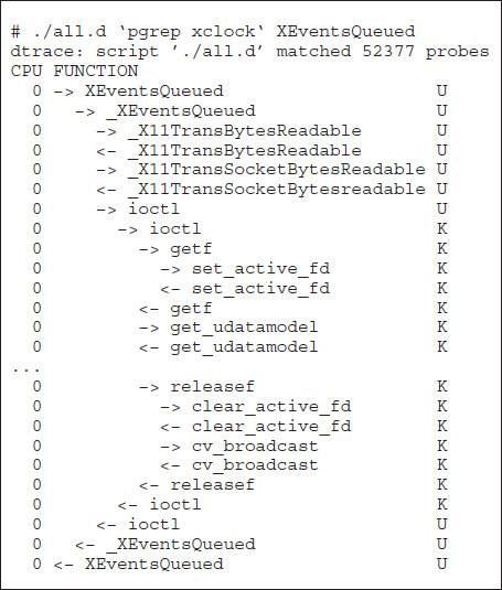
Figure 2.20 Solaris 10 dtrace follows a system call within the kernel.
In contrast, DTrace runs on production systems—systems that are running important or critical applications—and causes no harm to the system. It slows activities while enabled, but after execution it resets the system to its pre-debugging state. It is also a broad and deep tool. It can broadly debug everything happening in the system (both at the user and kernel levels and between the user and kernel layers). It can also delve deep into code, showing individual CPU instructions or kernel subroutine activities.
DTrace is composed of a compiler, a framework, providers of probes written within that framework, and consumers of those probes. DTrace providers create probes. Kernel structures exist to keep track of all probes that the providers have created. The probes are stored in a hash-table data structure that is hashed by name and indexed according to unique probe identifiers. When a probe is enabled, a bit of code in the area to be probed is rewritten to call dtrace_probe(probe identifier) and then continue with the code's original operation. Different providers create different kinds of probes. For example, a kernel system-call probe works differently from a user-process probe, and that is different from an I/O probe.
DTrace features a compiler that generates a byte code that is run in the kernel. This code is assured to be “safe” by the compiler. For example, no loops are allowed, and only specific kernel state modifications are allowed when specifically requested. Only users with DTrace “privileges” (or “root” users) are allowed to use DTrace, as it can retrieve private kernel data (and modify data if requested). The generated code runs in the kernel and enables probes. It also enables consumers in user mode and enables communications between the two.
A DTrace consumer is code that is interested in a probe and its results. A consumer requests that the provider create one or more probes. When a probe fires, it emits data that are managed by the kernel. Within the kernel, actions called enabling control blocks, or ECBs, are performed when probes fire. One probe can cause multiple ECBs to execute if more than one consumer is interested in that probe. Each ECB contains a predicate (“if statement”) that can filter out that ECB. Otherwise, the list of actions in the ECB is executed. The most common action is to capture some bit of data, such as a variable's value at that point of the probe execution. By gathering such data, a complete picture of a user or kernel action can be built. Further, probes firing from both user space and the kernel can show how a user-level action caused kernel-level reactions. Such data are invaluable for performance monitoring and code optimization.
Once the probe consumer terminates, its ECBs are removed. If there are no ECBs consuming a probe, the probe is removed. That involves rewriting the code to remove the dtrace_probe() call and put back the original code. Thus, before a probe is created and after it is destroyed, the system is exactly the same, as if no probing occurred.
DTrace takes care to assure that probes do not use too much memory or CPU capacity, which could harm the running system. The buffers used to hold the probe results are monitored for exceeding default and maximum limits. CPU time for probe execution is monitored as well. If limits are exceeded, the consumer is terminated, along with the offending probes. Buffers are allocated per CPU to avoid contention and data loss.
An example of D code and its output shows some of its utility. The following program shows the DTrace code to enable scheduler probes and record the amount of CPU time of each process running with user ID 101 while those probes are enabled (that is, while the program runs):
sched:::on-cpu
uid == 101
{
  self->ts = timestamp;
}

sched:::off-cpu
self->ts
{
  @time[execname] = sum(timestamp - self->ts);
  self->ts = 0;
}
The output of the program, showing the processes and how much time (in nanoseconds) they spend running on the CPUs, is shown in Figure 2.21.
Because DTrace is part of the open-source OpenSolaris version of the Solaris 10 operating system, it has been added to other operating systems when those systems do not have conflicting license agreements. For example, DTrace has been added to Mac OS X and FreeBSD and will likely spread further due to its unique capabilities. Other operating systems, especially the Linux derivatives, are adding kernel-tracing functionality as well. Still other operating systems are beginning to include performance and tracing tools fostered by research at various institutions, including the Paradyn project.
Figure 2.21 Output of the D code.
2.9 Operating-System Generation
It is possible to design, code, and implement an operating system specifically for one machine at one site. More commonly, however, operating systems are designed to run on any of a class of machines at a variety of sites with a variety of peripheral configurations. The system must then be configured or generated for each specific computer site, a process sometimes known as system generation SYSGEN.
The operating system is normally distributed on disk, on CD-ROM or DVD-ROM, or as an “ISO” image, which is a file in the format of a CD-ROM or DVD-ROM. To generate a system, we use a special program. This SYSGEN program reads from a given file, or asks the operator of the system for information concerning the specific configuration of the hardware system, or probes the hardware directly to determine what components are there. The following kinds of information must be determined.
- What CPU is to be used? What options (extended instruction sets, floating-point arithmetic, and so on) are installed? For multiple CPU systems, each CPU may be described.
- How will the boot disk be formatted? How many sections, or “partitions,” will it be separated into, and what will go into each partition?
- How much memory is available? Some systems will determine this value themselves by referencing memory location after memory location until an “illegal address” fault is generated. This procedure defines the final legal address and hence the amount of available memory.
- What devices are available? The system will need to know how to address each device (the device number), the device interrupt number, the device's type and model, and any special device characteristics.
- What operating-system options are desired, or what parameter values are to be used? These options or values might include how many buffers of which sizes should be used, what type of CPU-scheduling algorithm is desired, what the maximum number of processes to be supported is, and so on.
Once this information is determined, it can be used in several ways. At one extreme, a system administrator can use it to modify a copy of the source code of the operating system. The operating system then is completely compiled. Data declarations, initializations, and constants, along with conditional compilation, produce an output-object version of the operating system that is tailored to the system described.
At a slightly less tailored level, the system description can lead to the creation of tables and the selection of modules from a precompiled library. These modules are linked together to form the generated operating system. Selection allows the library to contain the device drivers for all supported I/O devices, but only those needed are linked into the operating system. Because the system is not recompiled, system generation is faster, but the resulting system may be overly general.
At the other extreme, it is possible to construct a system that is completely table driven. All the code is always part of the system, and selection occurs at execution time, rather than at compile or link time. System generation involves simply creating the appropriate tables to describe the system.
The major differences among these approaches are the size and generality of the generated system and the ease of modifying it as the hardware configuration changes. Consider the cost of modifying the system to support a newly acquired graphics terminal or another disk drive. Balanced against that cost, of course, is the frequency (or infrequency) of such changes.
2.10 System Boot
After an operating system is generated, it must be made available for use by the hardware. But how does the hardware know where the kernel is or how to load that kernel? The procedure of starting a computer by loading the kernel is known as booting the system. On most computer systems, a small piece of code known as the bootstrap program or bootstrap loader locates the kernel, loads it into main memory, and starts its execution. Some computer systems, such as PCs, use a two-step process in which a simple bootstrap loader fetches a more complex boot program from disk, which in turn loads the kernel.
When a CPU receives a reset event—for instance, when it is powered up or rebooted—the instruction register is loaded with a predefined memory location, and execution starts there. At that location is the initial bootstrap program. This program is in the form of read-only memory (ROM), because the RAM is in an unknown state at system startup. ROM is convenient because it needs no initialization and cannot easily be infected by a computer virus.
The bootstrap program can perform a variety of tasks. Usually, one task is to run diagnostics to determine the state of the machine. If the diagnostics pass, the program can continue with the booting steps. It can also initialize all aspects of the system, from CPU registers to device controllers and the contents of main memory. Sooner or later, it starts the operating system.
Some systems—such as cellular phones, tablets, and game consoles—store the entire operating system in ROM. Storing the operating system in ROM is suitable for small operating systems, simple supporting hardware, and rugged operation. A problem with this approach is that changing the bootstrap code requires changing the ROM hardware chips. Some systems resolve this problem by using erasable programmable read-only memory (EPROM), which is read-only except when explicitly given a command to become writable. All forms of ROM are also known as firmware, since their characteristics fall somewhere between those of hardware and those of software. A problem with firmware in general is that executing code there is slower than executing code in RAM. Some systems store the operating system in firmware and copy it to RAM for fast execution. A final issue with firmware is that it is relatively expensive, so usually only small amounts are available.
For large operating systems (including most general-purpose operating systems like Windows, Mac OS X, and UNIX) or for systems that change frequently, the bootstrap loader is stored in firmware, and the operating system is on disk. In this case, the bootstrap runs diagnostics and has a bit of code that can read a single block at a fixed location (say block zero) from disk into memory and execute the code from that boot block. The program stored in the boot block may be sophisticated enough to load the entire operating system into memory and begin its execution. More typically, it is simple code (as it fits in a single disk block) and knows only the address on disk and length of the remainder of the bootstrap program. GRUB is an example of an open-source bootstrap program for Linux systems. All of the disk-bound bootstrap, and the operating system itself, can be easily changed by writing new versions to disk. A disk that has a boot partition (more on that in Section 10.5.1) is called a boot disk or system disk.
Now that the full bootstrap program has been loaded, it can traverse the file system to find the operating system kernel, load it into memory, and start its execution. It is only at this point that the system is said to be running.
2.11 Summary
Operating systems provide a number of services. At the lowest level, system calls allow a running program to make requests from the operating system directly. At a higher level, the command interpreter or shell provides a mechanism for a user to issue a request without writing a program. Commands may come from files during batch-mode execution or directly from a terminal or desktop GUI when in an interactive or time-shared mode. System programs are provided to satisfy many common user requests.
The types of requests vary according to level. The system-call level must provide the basic functions, such as process control and file and device manipulation. Higher-level requests, satisfied by the command interpreter or system programs, are translated into a sequence of system calls. System services can be classified into several categories: program control, status requests, and I/O requests. Program errors can be considered implicit requests for service.
The design of a new operating system is a major task. It is important that the goals of the system be well defined before the design begins. The type of system desired is the foundation for choices among various algorithms and strategies that will be needed.
Throughout the entire design cycle, we must be careful to separate policy decisions from implementation details (mechanisms). This separation allows maximum flexibility if policy decisions are to be changed later.
Once an operating system is designed, it must be implemented. Operating systems today are almost always written in a systems-implementation language or in a higher-level language. This feature improves their implementation, maintenance, and portability.
A system as large and complex as a modern operating system must be engineered carefully. Modularity is important. Designing a system as a sequence of layers or using a microkernel is considered a good technique. Many operating systems now support dynamically loaded modules, which allow adding functionality to an operating system while it is executing. Generally, operating systems adopt a hybrid approach that combines several different types of structures.
Debugging process and kernel failures can be accomplished through the use of debuggers and other tools that analyze core dumps. Tools such as DTrace analyze production systems to find bottlenecks and understand other system behavior.
To create an operating system for a particular machine configuration, we must perform system generation. For the computer system to begin running, the CPU must initialize and start executing the bootstrap program in firmware. The bootstrap can execute the operating system directly if the operating system is also in the firmware, or it can complete a sequence in which it loads progressively smarter programs from firmware and disk until the operating system itself is loaded into memory and executed.
Practice Exercises
2.1 What is the purpose of system calls?
2.2 What are the five major activities of an operating system with regard to process management?
2.3 What are the three major activities of an operating system with regard to memory management?
2.4 What are the three major activities of an operating system with regard to secondary-storage management?
2.5 What is the purpose of the command interpreter? Why is it usually separate from the kernel?
2.6 What system calls have to be executed by a command interpreter or shell in order to start a new process?
2.7 What is the purpose of system programs?
2.8 What is the main advantage of the layered approach to system design? What are the disadvantages of the layered approach?
2.9 List five services provided by an operating system, and explain how each creates convenience for users. In which cases would it be impossible for user-level programs to provide these services? Explain your answer.
2.10 Why do some systems store the operating system in firmware, while others store it on disk?
2.11 How could a system be designed to allow a choice of operating systems from which to boot? What would the bootstrap program need to do?
Exercises
2.12 The services and functions provided by an operating system can be divided into two main categories. Briefly describe the two categories, and discuss how they differ.
2.13 Describe three general methods for passing parameters to the operating system.
2.14 Describe how you could obtain a statistical profile of the amount of time spent by a program executing different sections of its code. Discuss the importance of obtaining such a statistical profile.
2.15 What are the five major activities of an operating system with regard to file management?
2.16 What are the advantages and disadvantages of using the same system-call interface for manipulating both files and devices?
2.17 Would it be possible for the user to develop a new command interpreter using the system-call interface provided by the operating system?
2.18 What are the two models of interprocess communication? What are the strengths and weaknesses of the two approaches?
2.19 Why is the separation of mechanism and policy desirable?
2.20 It is sometimes difficult to achieve a layered approach if two components of the operating system are dependent on each other. Identify a scenario in which it is unclear how to layer two system components that require tight coupling of their functionalities.
2.21 What is the main advantage of the microkernel approach to system design? How do user programs and system services interact in a microkernel architecture? What are the disadvantages of using the microkernel approach?
2.22 What are the advantages of using loadable kernel modules?
2.23 How are iOS and Android similar? How are they different?
2.24 Explain why Java programs running on Android systems do not use the standard Java API and virtual machine.
2.25 The experimental Synthesis operating system has an assembler incorporated in the kernel. To optimize system-call performance, the kernel assembles routines within kernel space to minimize the path that the system call must take through the kernel. This approach is the antithesis of the layered approach, in which the path through the kernel is extended to make building the operating system easier. Discuss the pros and cons of the Synthesis approach to kernel design and system-performance optimization.
Programming Problems
2.26 In Section 2.3, we described a program that copies the contents of one file to a destination file. This program works by first prompting the user for the name of the source and destination files. Write this program using either the Windows or POSIX API. Be sure to include all necessary error checking, including ensuring that the source file exists.
Once you have correctly designed and tested the program, if you used a system that supports it, run the program using a utility that traces system calls. Linux systems provide the strace utility, and Solaris and Mac OS X systems use the dtrace command. As Windows systems do not provide such features, you will have to trace through the Windows version of this program using a debugger.
Programming Projects
Linux Kernel Modules
In this project, you will learn how to create a kernel module and load it into the Linux kernel. The project can be completed using the Linux virtual machine that is available with this text. Although you may use an editor to write these C programs, you will have to use the terminal application to compile the programs, and you will have to enter commands on the command line to manage the modules in the kernel.
As you'll discover, the advantage of developing kernel modules is that it is a relatively easy method of interacting with the kernel, thus allowing you to write programs that directly invoke kernel functions. It is important for you to keep in mind that you are indeed writing kernel code that directly interacts with the kernel. That normally means that any errors in the code could crash the system! However, since you will be using a virtual machine, any failures will at worst only require rebooting the system.
Part I—Creating Kernel Modules
The first part of this project involves following a series of steps for creating and inserting a module into the Linux kernel.
You can list all kernel modules that are currently loaded by entering the command
lsmod
This command will list the current kernel modules in three columns: name, size, and where the module is being used.
The following program (named simple.c and available with the source code for this text) illustrates a very basic kernel module that prints appropriate messages when the kernel module is loaded and unloaded.
#include <linux/init.h>
#include <linux/kernel.h>
#include <linux/module.h>

/* This function is called when the module is loaded. */
int simple_init(void)
{
  printk(KERN_INFO “Loading Module
”);

  return 0;
}

/* This function is called when the module is removed. */
void simple_exit(void)
{
  printk(KERN_INFO “Removing Module
”);
}

/* Macros for registering module entry and exit points. */
module_init(simple_init);
module_exit(simple_exit);

MODULE_LICENSE(“GPL”);
MODULE_DESCRIPTION(“Simple Module”);
MODULE_AUTHOR(“SGG”);
The function simple_init() is the module entry point, which represents the function that is invoked when the module is loaded into the kernel. Similarly, the simple_exit() function is the module exit point—the function that is called when the module is removed from the kernel.
The module entry point function must return an integer value, with 0 representing success and any other value representing failure. The module exit point function returns void. Neither the module entry point nor the module exit point is passed any parameters. The two following macros are used for registering the module entry and exit points with the kernel:
module_init()

module_exit()
Notice how both the module entry and exit point functions make calls to the printk() function. printk() is the kernel equivalent of printf(), yet its output is sent to a kernel log buffer whose contents can be read by the dmesg command. One difference between printf() and printk() is that printk() allows us to specify a priority flag whose values are given in the <linux/printk.h> include file. In this instance, the priority is KERN_INFO, which is defined as an informational message.
The final lines—MODULE_LICENSE(), MODULE_DESCRIPTION(), and MODULE_AUTHOR()—represent details regarding the software license, description of the module, and author. For our purposes, we do not depend on this information, but we include it because it is standard practice in developing kernel modules.
This kernel module simple.c is compiled using the Makefile accompanying the source code with this project. To compile the module, enter the following on the command line:
make
The compilation produces several files. The file simple.ko represents the compiled kernel module. The following step illustrates inserting this module into the Linux kernel.
Loading and Removing Kernel Modules
Kernel modules are loaded using the insmod command, which is run as follows:
sudo insmod simple.ko
To check whether the module has loaded, enter the lsmod command and search for the module simple. Recall that the module entry point is invoked when the module is inserted into the kernel. To check the contents of this message in the kernel log buffer, enter the command
dmesg
You should see the message “Loading Module.”
Removing the kernel module involves invoking the rmmod command (notice that the .ko suffix is unnecessary):
sudo rmmod simple
Be sure to check with the dmesg command to ensure the module has been removed.
Because the kernel log buffer can fill up quickly, it often makes sense to clear the buffer periodically. This can be accomplished as follows:
sudo dmesg -c
Proceed through the steps described above to create the kernel module and to load and unload the module. Be sure to check the contents of the kernel log buffer using dmesg to ensure you have properly followed the steps.
Part II—Kernel Data Structures
The second part of this project involves modifying the kernel module so that it uses the kernel linked-list data structure.
In Section 1.10, we covered various data structures that are common in operating systems. The Linux kernel provides several of these structures. Here, we explore using the circular, doubly linked list that is available to kernel developers. Much of what we discuss is available in the Linux source code—in this instance, the include file <linux/list.h>—and we recommend that you examine this file as you proceed through the following steps.
Initially, you must define a struct containing the elements that are to be inserted in the linked list. The following C struct defines birthdays:
struct birthday {
  int day;
  int month;
  int year;
  struct list_head list;
}
Notice the member struct list_head list. The list_head structure is defined in the include file <linux/types.h>. Its intention is to embed the linked list within the nodes that comprise the list. This list_head structure is quite simple—it merely holds two members, next and prev, that point to the next and previous entries in the list. By embedding the linked list within the structure, Linux makes it possible to manage the data structure with a series of macro functions.
Inserting Elements into the Linked List
We can declare a list_head object, which we use as a reference to the head of the list by using the LIST_HEAD() macro
static LIST_HEAD(birthday_list);
This macro defines and initializes the variable birthday_list, which is of type struct list_head.
We create and initialize instances of struct birthday as follows:
struct birthday *person;

person = kmalloc(sizeof(*person), GFP_KERNEL);
person->day = 2;
person->month= 8;
person->year = 1995;
INIT_LIST_HEAD(&person->list);
The kmalloc() function is the kernel equivalent of the user-level malloc() function for allocating memory, except that kernel memory is being allocated. (The GFP_KERNEL flag indicates routine kernel memory allocation.) The macro INIT_LIST_HEAD() initializes the list member in struct birthday. We can then add this instance to the end of the linked list using the list_add_tail() macro:
list_add_tail(&person->list, &birthday_list);
Traversing the Linked List
Traversing the list involves using the list_for_each_entry() Macro, which accepts three parameters:
- A pointer to the structure being iterated over
- A pointer to the head of the list being iterated over
- The name of the variable containing the list_head structure
The following code illustrates this macro:
struct birthday *ptr;

list_for_each entry(ptr, &birthday_list, list) {
  /* on each iteration ptr points */
  /* to the next birthday struct */
}
Removing Elements from the Linked List
Removing elements from the list involves using the list_del() macro, which is passed a pointer to struct list_head
list_del(struct list_head *element)
This removes element from the list while maintaining the structure of the remainder of the list.
Perhaps the simplest approach for removing all elements from a linked list is to remove each element as you traverse the list. The macro list_for_each_entry_safe() behaves much like list_for_each_entry() except that it is passed an additional argument that maintains the value of the next pointer of the item being deleted. (This is necessary for preserving the structure of the list.) The following code example illustrates this macro:
struct birthday *ptr, *next

list_for_each_entry_safe(ptr, next,&birthday_list,list) {
  /* on each iteration ptr points */
  /* to the next birthday struct */
  list_del(&ptr->list);
  kfree(ptr);
}
Notice that after deleting each element, we return memory that was previously allocated with kmalloc() back to the kernel with the call to kfree(). Careful memory management—which includes releasing memory to prevent memory leaks—is crucial when developing kernel-level code.
Part II Assignment
In the module entry point, create a linked list containing five struct birthday elements. Traverse the linked list and output its contents to the kernel log buffer. Invoke the dmesg command to ensure the list is properly constructed once the kernel module has been loaded.
In the module exit point, delete the elements from the linked list and return the free memory back to the kernel. Again, invoke the dmesg command to check that the list has been removed once the kernel module has been unloaded.
Bibliographical Notes
[Dijkstra (1968)] advocated the layered approach to operating-system design. [Brinch-Hansen (1970)] was an early proponent of constructing an operating system as a kernel (or nucleus) on which more complete systems could be built. [Tarkoma and Lagerspetz (2011)] provide an overview of various mobile operating systems, including Android and iOS.
MS-DOS, Version 3.1, is described in [Microsoft (1986)]. Windows NT and Windows 2000 are described by [Solomon (1998)] and [Solomon and Russinovich (2000)]. Windows XP internals are described in [Russinovich and Solomon (2009)]. [Hart (2005)] covers Windows systems programming in detail. BSD UNIX is described in [McKusick et al. (1996)]. [Love (2010)] and [Mauerer (2008)] thoroughly discuss the Linux kernel. In particular, [Love (2010)] covers Linux kernel modules as well as kernel data structures. Several UNIX systems—including Mach—are treated in detail in [Vahalia (1996)]. Mac OS X is presented at http://www.apple.com/macosx and in [Singh (2007)]. Solaris is fully described in [McDougall and Mauro (2007)].
DTrace is discussed in [Gregg and Mauro (2011)]. The DTrace source code is available at http://src.opensolaris.org/source/.
Bibliography
[Brinch-Hansen (1970)] P. Brinch-Hansen, “The Nucleus of a Multiprogramming System”, Communications of the ACM, Volume 13, Number 4 (1970), pages 238–241 and 250.
[Dijkstra (1968)] E. W. Dijkstra, “The Structure of the THE Multiprogramming System”, Communications of the ACM, Volume 11, Number 5 (1968), pages 341–346.
[Gregg and Mauro (2011)] B. Gregg and J. Mauro, DTrace—Dynamic Tracing in Oracle Solaris, Mac OS X, and FreeBSD, Prentice Hall (2011).
[Hart (2005)] J. M. Hart, Windows System Programming, Third Edition, Addison-Wesley (2005).
[Love (2010)] R. Love, Linux Kernel Development, Third Edition, Developer's Library (2010).
[Mauerer (2008)] W. Mauerer, Professional Linux Kernel Architecture, John Wiley and Sons (2008).
[McDougall and Mauro (2007)] R. McDougall and J. Mauro, Solaris Internals, Second Edition, Prentice Hall (2007).
[McKusick et al. (1996)] M. K. McKusick, K. Bostic, and M. J. Karels, The Design and Implementation of the 4.4 BSD UNIX Operating System, John Wiley and Sons (1996).
[Microsoft (1986)] Microsoft MS-DOS User's Reference and Microsoft MS-DOS Programmer's Reference. Microsoft Press (1986).
[Russinovich and Solomon (2009)] M. E. Russinovich and D. A. Solomon, Windows Internals: Including Windows Server 2008 and Windows Vista, Fifth Edition, Microsoft Press (2009).
[Singh (2007)] A. Singh, Mac OS X Internals: A Systems Approach, Addison-Wesley (2007).
[Solomon (1998)] D. A. Solomon, Inside Windows NT, Second Edition, Microsoft Press (1998).
[Solomon and Russinovich (2000)] D. A. Solomon and M. E. Russinovich, Inside Microsoft Windows 2000, Third Edition, Microsoft Press (2000).
[Tarkoma and Lagerspetz (2011)] S. Tarkoma and E. Lagerspetz, “Arching over the Mobile Computing Chasm: Platforms and Runtimes”, IEEE Computer, Volume 44, (2011), pages 22–28.
[Vahalia (1996)] U. Vahalia, Unix Internals: The New Frontiers, Prentice Hall (1996).