2

–––––––––––––––––––––––

Reliable Minimum Connected Dominating Sets for Topology Control in Probabilistic Wireless Sensor Networks

Jing (Selena) He, Shouling Ji, Yi Pan, and Yingshu Li

2.1   TOPOLOGY CONTROL IN WIRELESS SENSOR NETWORKS (WSNs)

To ensure sufficient coverage of an area or to protect against node failures, one major characteristic of WSNs is the possibility of deploying many redundant nodes in a small area. These are clear advantages of a dense network deployment; however, there are also disadvantages. To be specific, in a relatively crowded network, many typical wireless networking problems are aggravated by the large number of neighbors, such as many nodes interfering with each other. In order to avoid too many interferences, nodes might use short transmission power to talk to nearby nodes directly; thus, routing protocols might have to recompute routes even if only small node movements have happened [1].

Some of these problems can be overcome by topology-control techniques. Instead of using the possible connectivity of a network to its maximum possible extent, a deliberate choice is made to restrict the topology of the network. The topology of a network is determined by the subset of active nodes and the set of active links along which direct communication can occur. Formally speaking, a topology-control algorithm takes a graph G = (V, E) representing the network, where V is the set of all nodes in the network and there is an edge (v₁, v₂) ∈ E ⊆ V² if and only if nodes v₁ and v₂ can directly communicate with each other. All active nodes form an induced graph A = (V_A, E_A), such that V_A ⊆ V and E_A⊆ E.

2.1.1   Options for Topology Control

To compute an induced graph A out of a graph G representing the original network G, a topology-control algorithm has a few options [1]:

• The set of active nodes can be reduced (V_T ⊂ V) by periodically switching on/off some nodes in G.
• The set of active links/the set of neighbors for a node can be controlled. Instead of using all links in the network, some links can be disregarded and communication can be restricted to crucial links. When a flat network topology (all nodes are considered equal) is desired, the set of neighbors of a node can be reduced by simply not communicating with some neighbors. One possible approach to choose neighbors for a WSN is to limit a node's transmission range—typically by power control.
• Active links/neighbors can also be rearranged in a hierarchical network topology where some nodes assume special roles.

One example, illustrated in Figure 2.1, is to select some nodes as a virtual backbone (VB) for the network and to only use the links within this backbone and direct links from other nodes to the backbone. To do so, the backbone has to form a dominating set (DS). Formally speaking, a DS is a subset D ⊂ V such that all nodes in V are either in D itself or are one-hop neighbors of some node d ∈ D (i.e., ∀ v ∈ V: v ∈ D ∨ ∃ d ∈ D: (v, d) ∈ E). Then, only the links between nodes of the DS or between other nodes and a member of the active set are maintained. For a backbone to be useful, it should be connected. Hence, a connected dominating set (CDS) should always be used as a VB in WSNs.

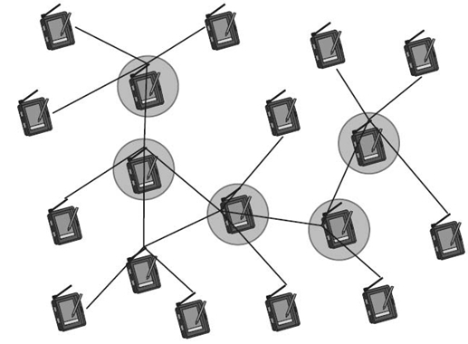
Figure 2.1. Restricting the topology by using dominating sets.

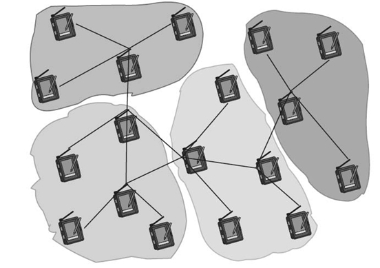
Figure 2.2. Using clusters to partition a graph.

A related but slightly different idea is to partition the network into clusters, illustrated in Figure 2.2. Clusters are subsets of nodes such that, for each cluster, certain conditions hold. The most typical problem formulation is to find clusters with cluster heads, which is a representative of a cluster such that each node is only one hop away from its cluster head.

In summary, there are three main options for topology control: flat networks with a special attention to power control on the one hand, hierarchical networks with backbones or clusters on the other hand.

2.1.2   Measurements of Topology-Control Algorithms

There are a few basic metrics to judge the efficiency and quality of a topology-control algorithm [2]:

• Connectivity. Topology control should not disconnect a connected graph G.
• Stretch Factors. Removing links from a graph will likely increase the length of a path between any two nodes, u and v. The hop stretch factor is defined as the worst increase in path length for any pair of nodes u and v between the original graph G and the topology-controlled path P. Formally,

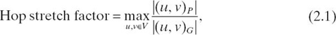
where (u, v)_G is the shortest path in graph G and |(u, v)_G| is its length. Similarly, the energy stretch factor can be defined:

where E_G (u, v) is the energy consumed along the most energy-efficient path in graph G. Clearly, topology-control algorithms with small stretch factors are desirable.

• Graph Metrics. A small number of edges in induced graph A and a low maximum degree for each node in A.
• Throughput. The reduced network topology should be able to sustain an amount of traffic comparable to that of the original network.
• Robustness to Mobility. When neighborhood relationships are changed in the original graph, other nodes might have to change their topology information.
• Algorithm Overhead. Low number of additional messages, low computational overhead. Also, distributed implementation is more practical and more desired.

In the present context of WSNs, connectivity is perhaps the most important characteristic of a topology-control algorithm. In this work, we focus on the CDS-based topology control.

2.2   DS-BASED TOPOLOGY CONTROL

2.2.1   Motivation

Different from wired networks, the topology of a WSN may change from time to time, and the energy of nodes is very limited and irreplaceable. Therefore, designing an energy-efficient communication scheme for WSNs is one of the most important issues that has a significant impact on the network performance. The effectiveness of many communication primitives for WSNs, such as routing [3, 4], multicast/broadcast [5, 6], and service discovery [7], relies heavily on the availability of a VB. A CDS typically serves as a VB of a WSN. A CDS is defined as a subset of nodes in a WSN such that each node in the network is either in the set or adjacent to some node in the set, and the induced graph by the nodes in the set is connected. The nodes in a CDS are called dominators, otherwise, dominatees. In a WSN with a CDS as its VB, dominatees only forward their data to their connected dominators. In addition to communication schemes, a CDS has many other applications, such as topology control [8], coverage [9, 10], data collection [11‒13], data aggregation [14], and query scheduling [15]. Clearly, the benefits of a CDS can be magnified by making its size (the number of the nodes in the CDS) smaller. In general, the smaller the CDS is, the less communication and storage overhead are incurred. Hence, it is desirable to build a minimum-sized connected dominating set (MCDS).

Ever since the idea of employing a CDS for WSNs was introduced [16], a huge amount of effort has been made to find different CDSs for different applications, especially MCDSs. They can be classified into the following four categories based on the network information they use:

• centralized algorithms
• subtraction-based distributed algorithms
• distributed algorithms using a single leader
• distributed algorithms using multiple leaders.

We use n to denote the number of sensors in a WSN, Δ to denote the maximum degree of nodes in the graph representing a WSN, and opt to denote the size of any optimal MCDS.

2.2.2   Centralized Algorithms

Guha and Khuller [17] first proposed two centralized greedy algorithms with performance ratios of 2(H (Δ) + 1) and H (Δ) + 2, respectively, where H (.) is a harmonic function. The greedy function is based on the number of white neighbors of each node. At each step, the one with the largest such number becomes a dominator.

Due to the instability of network topology in WSNs, it is necessary to update topology information periodically. Therefore, many distributed algorithms are proposed. These distributed algorithms can be classified into two categories: subtraction-based and addition-based algorithms. The subtraction-based algorithms begin with the set of all the nodes in a network, then remove some nodes according to predefined rules to obtain a CDS. The addition-based CDS algorithms start from a subset of nodes (usually disconnected), then include additional nodes to form a CDS. Depending on the type of the initial subset, the addition-based CDS algorithms can be further divided into single-leader and multiple-leader algorithms.

2.2.3   Subtraction-Based Distributed Algorithms for CDSs

Wu and Li [18] first proposed a completely distributed algorithm to obtain a CDS. The CDS construction procedure consists of two stages. In the first stage, each node collects its neighboring information by exchanging a message with the one-hop neighbors. If a node finds that there is a direct link between any pair of its one-hop neighbors, it removes itself from the CDS. In the second stage, additional heuristic rules are applied to further reduce the size of the CDS. Wu's algorithm [18] uses rule 1 and rule 2, where a node is removed from the CDS, if all its neighbors are covered by its one or two direct neighbors. Later, Dai's work [19] generalizes this as rule k, in which coverage is defined by an arbitrary number of connected neighbors. Dai's algorithm is reduced to Wu's algorithm when k is 1 or 2.

2.2.4   Addition-Based Distributed Algorithms for CDSs

Single-leader distributed algorithms for CDSs use one initiator to initialize the distributed algorithms. Usually, a base station could be the initiator for constructing CDSs in WSNs. In these distributed algorithms, a spanning tree rooted at the initiator is first constructed, and then maximal independent sets (MISs) are identified layer by layer; finally, a set of connectors to connect the MISs is ascertained to form a CDS. Wan et al. [20] presented an ID-based distributed algorithm to construct a CDS using a single initiator. For unit disk graphs (UDGs), Wan et al.'s [20] approach guarantees that the approximation factor on the size of a CDS is at most 8opt + 1. The algorithm has O(n) time complexity and O(n log n) message complexity. Subsequently, the approximation factor on the size of a CDS was improved in another work reported by Cardei et al. [21], in which the authors used the degree-based heuristic and degree-aware optimization to identify Steiner nodes as the connectors in the CDS construction. The approximation factor on the size of a CDS is improved to 8opt, while this distributed algorithm has O(n) message complexity and O(Δn) time complexity. Later, Li et al. [22] reported a better approximation factor of 5.8 + ln 4 by constructing a Steiner tree when connecting all the nodes in the MISs.

Distributed algorithms with multiple leaders do not require an initiator to construct a CDS. Alzoubi et al.'s technique [23] first constructs an MIS using a distributed approach without a leader or tree construction and then interconnects these MIS nodes to get a CDS. Li et al. proposed a distributed algorithm r-CDS in Reference 24, whose performance ratio is 172. r-CDS is a completely distributed one-phase algorithm where each node only needs to know the connectivity information within its two-hop-away neighborhood. An MIS is constructed based on each node's r value, which is defined as the number of this node's two-hop-away neighbors minus the degree of this node. The nodes with smaller r values are preferred to serve as MIS nodes. Adjih et al. [25] presented an approach for constructing an MCDS based on multipoint relay s (MPRs), but there is no approximation analysis of the algorithm yet. Recently, in Reference 26, another distributed algorithm was proposed whose performance ratio is 147. This algorithm contains three steps. Step 1 constructs a forest in which each tree is rooted at a node with the minimum ID among its one-hop-away neighbors. Step 2 collects the neighborhood information, which is used in step 3 to connect neighboring trees.

2.2.5   Other Algorithms

Because CDSs can benefit a lot from WSNs, a variety of other factors are considered when constructing CDSs. There are more than one CDS that can be found for each WSN. To conserve energy, all CDSs are constructed and each CDS serves as the VB duty cycled in Reference 27. For the sake of fault tolerance, k-connect m-DSs [28] are constructed, where k-connectivity means that between any pair of backbone nodes, there exist at least k independent paths, and m-dominating represents that every dominatee has at least m adjacent dominator neighbors. To minimize delivery delay, a special CDS problem—minimum routing cost connected dominating set (MOC-CDS) [29] is proposed, where each pair of nodes in MOC-CDS has the shortest path. The work [30] considers size, diameter, and average backbone path length (ABPL) of a CDS in order to construct a CDS with better quality. Recently, the authors in References 31‒33 take the load-balance factor into consideration when constructing an MCDS.

2.3   DETERMINISTIC WSNs AND PROBABILISTIC WSNs

WSNs are usually modeled using the deterministic network model (DNM) in recent literature. Under this model, there is a transmission radius of each node. According to this radius, any specific pair of nodes is always connected to be neighbors if their physical distance is less than this radius, while the rest of the pairs are always disconnected. The UDG model is a special case of the DNM model if all nodes have the same transmission radius. When all nodes are connected to each other, via a single-hop or multihop path, a WSN is said to have full connectivity. In most real applications, however, the DNM model cannot fully characterize the behavior of wireless links. This is mainly due to the transitional region phenomenon, which has been revealed by many empirical studies [34‒37]. Beyond the “always connected” region, there is a transitional region where a pair of nodes is probabilistically connected. Such pairs of nodes are not fully connected but are reachable via the so-called lossy links [37]. As reported in Reference [37], there are often many more lossy links than fully connected links in a WSN. Additionally, in a specific setup [38], more than 90% of the network links are lossy links. Therefore, their impact can hardly be neglected.

The employment of lossy links in WSNs is not straightforward since when the lossy links are employed, the WSN may have no guarantee of full network connectivity. When data transmissions are conducted over such topologies, it may degrade the node-to-node delivery ratio. Usually, a WSN has large node density and high data redundancy; thus, this certain degraded performance may be acceptable for many WSN applications. Therefore, as long as an expected percentage of the nodes can be reached, that is, the node-to-node delivery ratio satisfies some preset requirement, lossy links are tolerable in a WSN. In other words, full network connectivity is not always a necessity. Some applications can trade full network connectivity for a higher energy efficiency and larger network capacity [38].

All the above-mentioned existing works either consider to construct an MCDS under the DNM model, to design a routing protocol, or to investigate the topology control under the probabilistic network model (PNM). To our best knowledge, however, none of them attempts to construct an MCDS under the PNM model, which is more realistic. This is the major motivation of this research work. Genetic algorithms (GAs) are a family of computational models inspired by evolution, which have been applied in a quite broad range of NP-hard optimization problems [39‒42]. Therefore, a GA-based method, namely, reliable minimum-sized connected dominating set genetic algorithm (RMCDS-GA), is proposed in Section 2.5 to construct a reliable minimum-sized connected dominating set (RMCDS) under the PNM model. In RMCDS-GA, each possible CDS in a WSN is represented to be a chromosome (feasible/potential solution), and the fitness function is to evaluate the trade-off between the CDS reliability and the size of the CDS represented by each chromosome.

2.4   RELIABLE MCDS PROBLEM

2.4.1   Motivation Example

In order to well characterize a WSN with lossy links, we propose a new network model called the PNM. Under this model, in addition to the transmission radius, there is a transmission success ratio (TSR) associated with each link connecting a pair of nodes, which is used to indicate the probability that one node can successfully directly deliver a package to another. Obviously, the core issue under the PNM model is how to guarantee the node-to-node delivery ratio of all possible node pairs satisfying the user requirement, in other words, how to guarantee the transmission quality (TQ). For constructing an MCDS under the PNM model, we propose CDS reliability to measure its TQ. Given a PNM model, CDS reliability is defined as the minimum node-to-node delivery ratio between any pair of dominators. Thus, how to find an RMCDS under the PNM model is the major concern of this chapter. The objective is to seek an MCDS whose reliability satisfies a certain application dependent threshold denoted by σ (e.g., σ = 80%). If σ = 100%, finding an RMCDS under the PNM model is the same as the traditional MCDS problem under the DNM model. However, a traditional MCDS algorithm may not find an RMCDS under the PNM model. A counterexample is depicted in Figure 2.3. By the latest algorithm proposed in Reference 14, a spanning tree rooted at a specified initiator is first constructed, and then MISs are identified layer by layer. Finally, a set of connectors to connect the MISs is ascertained to form a CDS. According to the topology shown in Figure 2.3, the constructed CDS by Wan et al. [14] using s₄ as the initiator is D = {s₄, s₇, s₈}, whose reliability is 0.1. If the threshold σ = 0.7, the CDS D does not satisfy the constraint at all. The objective of our work is to find an MCDS whose reliability is greater than or equal to σ. One example of the satisfied RMCDS is D′ = {s₃, s₆, s₇} in Figure 2.3.

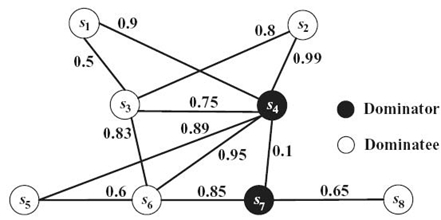
Figure 2.3. A wireless network under the PNM model.

The key challenge of finding an RMCDS under the PNM model is the computation of the CDS reliability. It is known that given a network topology, the calculation of the node-to-node delivery ratio is NP-hard when network broadcast is used. Indeed, according to the reliability theory [43], the node-to-node delivery ratio is not practically computable unless the network topology is basically series‒parallel, namely, the graph representing a WSN can be reduced to a single edge by series and parallel replacements. Nevertheless, most network topologies are not series‒parallel structures. Thus, instead of computing the accurate CDS reliability, we design a greedy-based algorithm to approximate the CDS reliability. Another challenge is to find an MCDS, which is also an NP-hard problem [44]. Intuitively, the smaller the CDS is, the lower the reliability of the CDS is. The key issue then becomes how to find a proper trade-off between the MCDS and the CDS reliability while satisfying the optimization constraint (i.e., the CDS reliability is no less than the threshold σ). To address this problem, we explore the GA optimization approach. GAs are numerical search tools that operate according to the procedures that resemble the principles of natural selection and genetics [45]. Because of their flexibility and widespread applicability, GAs have been successfully used in a wide variety of problems in several areas of WSNs [39‒42].

2.4.2   Assumptions

We assume a static WSN and all the nodes have the same transmission range. The transmission success ratio (TSR) associated with each link connecting a pair of nodes is available and fixed, which can be obtained by periodic Hello messages or can be predicted using link quality index (LQI) [46]. We also assume that the TSR values are fixed. This assumption is reasonable as many empirical studies have shown that LQI is pretty stable in a static environment [47]. Furthermore, no node failure is considered since it is equivalent to a link failure case. No duty cycle is considered either. We do not consider packet collisions or transmission congestion, which are left to the medium access control (MAC) layer. The degradation of the node-to-node delivery ratio is thus only due to the failure of wireless links.

2.4.3   Network Model

We assume a static WSN and all the nodes have the same transmission range. The transmission success ratio (TSR) associated with each link connecting a pair of nodes is available and fixed. Under the PNM, we model a WSN as an undirected graph G (V, E, (E)), where V is the set of n nodes, denoted by s₁, s₂,…, s_n; E is the set of m lossy links, ∀ u, v ∈ V; there exists an edge (u, v) in G if and only if (1) u and v are in each other's transmission range and (2) TSR(e = {u, v}) > 0, for each link e = {u, v} ∈ E, where TSR(e) indicates the probability that node u can successfully directly deliver a packet to node v; and P (E) = {< e, TSR(e) >| e ∈ E, 0 ≤ TSR(e) ≤ 1}. We assume edges are undirected (bidirectional), which means two linked nodes are able to transmit and receive information from each other with the same TSR value.

Because of the introduction of TSR(e), the traditional definition of the node neighborhood has changed. Hence, we first give the definition of the one-hop neighborhood and then extend it to the r-hop neighborhood.

Definition 2.1   One-Hop Neighborhood.  ∀ u∈ V, the one-hop neighborhood of node u is defined as

The physical meaning of one-hop neighborhood is the set of the nodes that can be directly reached from node u.

Definition 2.2   r-Hop Neighborhood. ∀ u ∈ V, the r-hop neighborhood of node u is defined as

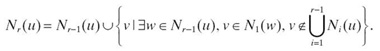
The physical meaning of the r-hop neighborhood is the set of nodes that can be reached from node u by passing maximum r number of edges.

Definition 2.3   Θk(i). Given a source node u, its k-hop and (k−1)-hop neighborhood N_k(u), N_k–1(u), for each i ∈ N_k(u), we denote Θ_k(i) as a set of edges that gives all the possible ways by which i can be reached from node i'∈ N_k–1(u):

Definition 2.4   Node-to-Node Delivery Ratio. Given a source node u and a destination node v, one path between the node pair can be denoted by the edge permutation θ(u, v) = (e₁ , e₂,…, e_m), and the delivery ratio of the path is denoted by . Furthermore, we use Θ(u, v) to denote the set of all the possible ways by which node v can be reached from node u. The node-to-node delivery ratio from node u to node v is then defined as

Clearly, DR*(u, v) is equivalent to DR*(v, u)

Definition 2.5   CDS Reliability. Given a WSN represented by G(V, E, P(E)) under the PNM model, and its CDS denoted by D, the reliability of D is the minimum node-to-node delivery ratio between any pair of the nodes in the CDS; that is,

We use CDS reliability to measure the quality of a CDS constructed under the PNM model. By this definition, when a CDS D has a reliability satisfying a threshold σ (i.e., ≥σ), we can state that for any pair of the nodes in the CDS, the probability that they are connected is no less than the threshold.

According to the reliability theory [43], we know that the computation of the node-to-node delivery ratio is NP-hard. Therefore, the computation of the CDS reliability is also NP-hard. In summary, we claim that, given a WSN represented by G (V, E, P (E)) under the PNM model, a CDS for G denoted by D, and a predefined threshold σ ∈ (0, 1], it is NP-hard to verify whether ≥σ.

2.4.4   Problem Definition

Definition 2.6   RMCDS. Given a WSN represented by G(V, E, P(E)) under the PNM model, and a predefined threshold σ ∈ (0, 1], the RMCDS problem is to find u, a minimum-sized node set D ⊆ V, such that

1. The induced graph G [D] = (D, E'), where E' = {e|e = (u, v), u ∈ D, v ∈ D, (u, v)∈ E)}, is connected.
2. ∀ u ∈ V and u ∉ D, ∃ v ∈ D, such that (u, v) ∈ E.
3. R_D^* ≥σ.

We claim that the problem to construct an RMCDS for a WSN under the PNM model is NP-hard. It is easy to see that the traditional MCDS problem under the DNM model is a special case of the RMCDS problem. By setting the TSR values on all edges to 1, we are able to convert the RMCDS problem to the traditional MCDS problem under the DNM model. Thus, the RMCDS problem belongs to NP. The verification of the RMCDS problem needs to calculate the CDS reliability. It is an NP-hard problem, which is mentioned in Section 2.4.3. Therefore, the problem to construct an RMCDS for a WSN under the PNM model is NP-hard.

2.4.5   Remarks

As we already know, computing the node-to-node delivery ratio and the CDS reliability are NP-hard problems. Therefore, instead of computing the accurate node-to-node delivery ratio, we design a greedy-based algorithm to approximate the ratio denoted by DR(u, v). Based on the approximate node-to-node delivery ratio, we then calculate the approximate CDS reliability denoted by R_D. When there is no confusion, DR*(u, v) and DR(u, v), and R_D are interchangeable in the chapter.

Based on Definition 2.6, the key issue of the RMCDS problem is to seek a trade -off between the MCDS and the CDS reliability. GAs are population-based search algorithms that simulate biological evolution processes and have successfully solved a wide range of NP-hard optimization problems [39‒42]. In the following, algorithm RMCDS-GA is proposed to solve the RMCDS problem to search the feasible domain more effectively and to reduce the computation time.

2.5   A GA TO CONSTRUCT RMCDS-GA

2.5.1   GA Overview

GAs, first formalized as an optimization method by Holland [48], are search tools modeled after the genetic evolution of natural species. GAs encode a potential solution to a vector of independent variables called chromosomes. The independent variables consisting of chromosomes are called genes. Each gene encodes one component of the target problem. A binary coding is widely used nowadays. GAs differ from most optimization techniques because of their global searching effectuated by one population of solutions rather than from one single solution. Hence, a GA search starts with the creation of the first generation, a random initial population of chromosomes, that is, potential solutions to the problem. Then, these individuals in the first generation are evaluated in terms of their “fitness” values, that is, their corresponding objective function values. Based on their fitness values, a ranking of the individuals in the first generation is dynamically updated. Subsequently, the first generation is allowed to evolve in successive generations through the following steps:

1.  Reproduction. Selection of a pair of individuals in the current generation as parents. The ranking of individuals in the current generation is used in the selection procedure so that in the long run, the best individuals will have a greater probability of being selected as parents.

2.  Recombination. Crossover operation and mutation operation:

(a) Crossover is performed with a crossover probability, P_c, by selecting a random gene along the length of the parent chromosomes and swapping all the genes of the selected parent chromosomes after that point. The operation generates two new children chromosomes.

(b) Mutation is performed with a mutation probability, P_m, by flipping the value of one gene in the chromosomes (e.g., 0 becomes 1 and 1 becomes 0, if binary coding is used).

3.  Replacement. Utilization of the fittest individual to replace the worst individual of the current generation to create a new generation, so as to maintain the population number k a constant. Every time new children are generated by a GA, the fitness function is evaluated. And then a ranking of the individuals in the current generation is dynamically updated. The ranking is used in the replacement procedures to decide who among the parents and the children chromosomes should survive in the next population. This is to resemble the natural principles of the “survival of the fittest.”

GAs usually stop when a certain number of total generations denoted by G are reached.

Figure 2.4 shows the overview of the RMCDS - GA algorithm.

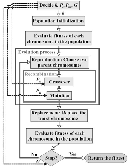
Figure 2.4. Procedure of RMCDS-GA.

One important feature of GAs that needs to be emphasized here is that the optimization performance of GAs depends mainly on the convergence time of the algorithm. When using GAs, sufficient genetic diversity among solutions in the population should be guaranteed. Lack of such diversity would lead to a reduction of the search space spanned by the GA. Consequently, the GA may prematurely converge to a local minimum because mediocre individuals are selected in the final generation. Alternatively, an excess of genetic diversity, especially at later generations, may lead to a degradation of the optimization performance. In other words, excess genetic diversity may result in very late or even no convergence. In this chapter, genetic diversity is maintained by the crossover, mutation operations and immigrant schemes. In the following part of this section, we will explain RMCDS-GA step by step.

2.5.2   Representation of Chromosomes

In the proposed RMCDS-GA, each node is mapped to a gene in the chromosome. A gene value indicates whether the node represented by this gene is a dominator or not. Hence, a chromosome is denoted as: C_i = (g₁, g₂,…, g_j,…, g_n), where 1 ≤ i ≤ k and k is the number of the chromosomes in the population; 1 ≤ j ≤ n and n is the total number of the nodes in a WSN:

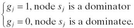
All the nodes with g_j = 1 form a CDS denoted by D = {s_j|g_j = 1, 1 ≤ j ≤ n}.

An example WSN under the PNM model is shown in Figure 2.3 to illustrate the encoding scheme. There are eight nodes and the CDS is D = {s₄, s₇}. Thus, the eight nodes can be encoded using eight genes in a chromosome, for example, C₁ = (g₁, g₂,…, g₈), and then set the values of genes representing the dominators to 1. Finally, the encoded chromosome is C₁ = (0, 0, 0, 1, 0, 0, 1, 0).

2.5.3   Population Initialization

According to the flowchart of the proposed RMCDS-GA shown in Figure 2.4, according to the proposed RMCDS-GA algorithm, after we decide the encoding scheme of the RMCDS problem, the first generation (a population with k chromosomes) should be created. This step is called population initialization in Figure 2.4. A general method to initialize the population is to explore the genetic diversity; that is, for each chromosome, all dominators are randomly generated. However, thedominators must form a CDS. Therefore, we start to create the first chromosome by running an existing MCDS method, for example, Wan's work [14], and then generate the population with k chromosomes by modifying the first chromosome. We call the procedure, generating the whole population by modifying one specific chromosome, inheritance population initialization (IPI).

An example is shown in Figure 2.3 to illustrate the IPI process. In Figure 2.3, the network and its CDS D₁ = {s₄, s₇} are given. The values on the edges are TSR values and black nodes are dominators. Furthermore, we assume the CDS is constructed by a traditional MCDS method. According to the encoding scheme mentioned in Section 2.5.2. C₁ = (0, 0, 0, 1, 0, 0, 1, 0) represents the CDS generated by Wan's work [14] shown in Figure 2.3. Subsequently, we need to generate more chromosomes based on the first chromosome. The IPI algorithm is summarized as follows:

1. Start from the node with the smallest ID; reduce one dominator each time from the original CDS D₁ represented by C₁. If the new obtained node set is still a CDS D_i, then encode it as a chromosome C_i and add it into the initial population. Otherwise, remove the node with the second smallest ID from the original CDS D₁ and make the same checking process as for the node with the smallest ID, repeating the process until no more new chromosomes can be created. The CDS shown in Figure 2.3 is an MCDS; that is, we cannot further reduce its size. Thus, we go to step 2.

2. If the size of the original CDS D₁ cannot be reduced, and the number of the generated chromosomes is less than k, then for all the existing chromosomes C₁, C₂,…, C_i do the following steps until k nonduplicated chromosomes are generated.

(a) Let t = 1.

(b) In the CDS D_t represented by the chromosome C_t, start from node u with the smallest ID and add one dominatee node in its one-hop neighborhood N₁ (u) by the order of its ID into the CDS each time. If the new obtained node sets form CDSs, then encode them as chromosomes and add them into the initial population. In Figure 2.5b, the node with the smallest ID is s₄ in D. Therefore, the chromosomes from C₂ to C₆ are generated by adding one node from set N₁ (s₄) = {s₁, s₂, s₃, s₅, s₆} each time.

(c) Move to the node with the second smallest ID in CDS D_t until every node in D_t is checked. In Figure 2.5b, the one-hop neighborhood of the node with the second smallest ID s₇ is N₁(s₇) = {s₆, s₈}. Since s₆ has already been marked as a dominator, we cannot add it to create a new CDS. By eliminating the duplicates, the chromosome C₇ is created.

(d) If all the dominators in the current D_t are checked, move to the next CDS by setting t = t + 1. Repeat the step from 2b to 2d.

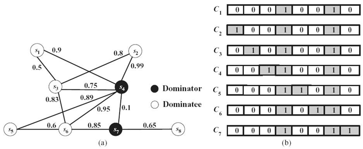
Figure 2.5. Illustration of population of initialization.

Since each node has two choices, to be a dominator or a dominatee, consequently, there are 2^n−|D| possible ways to create new chromosomes, where |D| is the size of the CDS denoted by D under the PNM model. Usually, k is much smaller than 2^n−|D|. Hence, the initial population C₁, C₂,…, C_k can be easily generated.

There are several merits that need to be pointed out here when using the above IPI algorithm to generate the initial population. First, we can guarantee every dominator set represented by a chromosome in the first generation is a CDS; that is, each chromosome in the initial population is a feasible solution of the RMCDS problem. Second, the critical nodes (cut nodes) are dominators encoded in each chromosome of the initial population. When performing crossover operations, the critical nodes are still dominators in the new offspring chromosome in the successive generations. Illustration examples will be shown in Section 2.5.6.1. Finally, the IPI stops when k chromosomes are generated. Actually, we can obtain more valid solutions by continuously running the IPI algorithm. As we already know, the population diversity plays an important role in the optimization performance of GAs. Therefore, the extra valid solutions generated by keeping running the IPI algorithm can be used in the replacement process to bring more population diversity in new generations. We will give a more detailed description of the replacement scheme in Section 2.5.6.3.

2.5.4   Fitness Function

Given a solution, its quality should be accurately evaluated by the fitness value, which is determined by the fitness function. In our algorithm, we aim to find an MCDS D whose reliability R_D should be greater than or equal to a preset threshold σ. Therefore, the fitness function of a chromosome C_i in the population is defined as

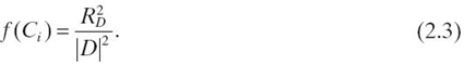
The purpose of rasing |D| and R_D to the power of 2 in Equation (2.3) is to enlarge the weight of the size of the CDS D. The denominator in Equation (2.3) needs to be minimized, while the numerator needs to be maximized. As a result, the fitness function value will be maximized.

As mentioned in the previous section, precisely calculating the CDS reliability is an NP-hard problem. According to Definition 2.5, we can easily compute the CDS reliability based on the node-to-node delivery ratio of all possible dominator pairs in the CDS. Therefore, we propose a greedy-based approximate algorithm to calculate the node-to-node delivery ratio. We adopt a greedy-based routing protocol, greedy perimeter stateless routing (GPSR) [49], to find the paths between all dominator pairs. In this work, we modified the greedy criterion to be the largest TSR values in one-hop neighborhoods based on GPSR.

For better understanding, we first illustrate the idea by an example and then summarize the whole process. For the chromosome C₂ shown in Figure 2.5b, the CDS represented by C₂ is D = {s₁, s₄, s₇}, in which there are three possible dominator pairs, that is, (s₁, s₄), (s₁, s₇), and (s₄, s₇). Assume the reliability threshold isσ = 60%. Clearly, the TSRs associated with the edges (s₁, s₄) and (s₄, s₇) are both greater than 60% in Figure 2.5; that is, TSR (e₁ = {s₁, s₄}) = 0.9 and TSR (e₂ = {s₄, s₇}) = 0.95. According to Definition 2.4, we know that DR(s₁, s₄) = 0.9 and DR(s₄, s₇) = 0.95, respectively. Therefore, the first greedy criterion comes out: The direct edges between sources and destinations with TSR values greater than δ have the highest priority to be chosen as the path between sources and destinations. Obviously, there is no direct edge between dominator pair (s₁, s₇). Thus, we need to find a multihop path between them. The search process starts from the destination s₇. The greedy criterion is based on the TSR values on the edges between s₇ and all its one-hop neighborhood N₁ (s₇) = {s₄, s₆, s₈}. Since TSR (e₂ = {s₄, s₇}) = 0.95 > 0.6 is the largest TSR value among all the nodes in N₁ (s₇), the edge e₂ = {s₄, s₇} is chosen. Subsequently, we keep searching froms₄. Apparently, TSR (e₃ = {s₂, s₄}) = 0.99> 0.6 is the highest TSR value on the edges from s₄to all the nodes in N₁ (s₄). However, based on the direct edge greedy criterion, that is, there is a direct edge between the sources₁and the current search nodes₄, therefore, e₁ = {s₁, s₄} is chosen. According to Definition 2.4, θ (s₁, s₇) = {e₁, e₂}, DR (s₁, s₇) = = 0.9 × 0.95 = 0.855. Finally, based on Definition 2.5, we know R (D) = min{DR (s₁, s₄), DR (s₁, s₇), DR (s₄, s 7)} = min{0.9, 0.855, 0.95} = 0.855. The fitness of C₂ can then be calculated using Equation (2.3), f (C₂) = 0.855² /3² = 0.081225.

2.5.5   Selection (Reproduction) Scheme

During the evolutionary process, election plays an important role in improving the average quality of the population by passing the high-quality chromosomes to the next generation. The selection operator is carefully formulated to ensure that better chromosomes of the population (with higher fitness values) have a greater probability of being selected for mating but that worse chromosomes of the population still have a small probability of being selected. Having some probability of choosing worse members is important to ensure that the search process is global and does not simply converge to the nearest local optimum. We adopt roulette wheel selection (RWS) since it is simple and effective. RWS stochastically selects individuals based on their fitness values f(C_i). A real-valued interval, S, is determined as the sum of the individuals'expected selection probabilities; that is,

where

Individuals are then mapped one to one into contiguous intervals in the range [0, S]. The size of each individual interval corresponds to the fitness value of the associated individual. The circumference of the roulette wheel is the sum of all fitness values of the individuals. The fittest chromosome occupies the largest interval, whereas the least fit has a correspondingly smaller interval within the roulette wheel. To select an individual, a random number is generated in the interval [0, S], and the individual whose segment spans the random number is selected. This process is repeated until a desired number of individuals have been selected.

TABLE 2.1. Fitness of Seven Chromosomes

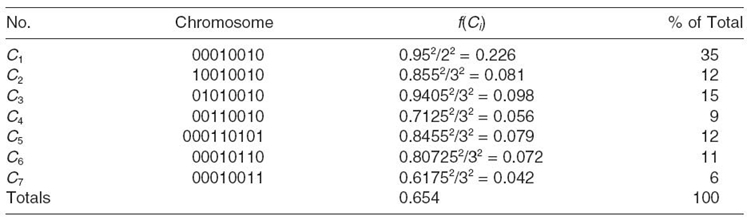
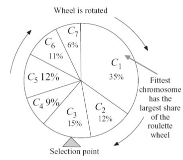
FIGURE 2.6. Roulette wheel selection.

We still use the WSN shown in Figure 2.5a to illustrate the RWS scheme. Table 2.1 lists a sample population of seven individuals (shown in Figure 2.5b). These individuals consist of 8-bit chromosomes. The fitness values are calculated by Equation (2.3). We can see from the table that C₁ is the fittest and C₇ is the weakest. Summing these fitness values, we can apportion a percentage total of fitness. This gives the strongest individual a value of 35% and the weakest 6%. These percentage fitness values can then be used to configure the roulette wheel (shown in Fig. 2.6). The number of times the roulette wheel is spun is equal to size of the population (i.e., k). As can be seen from the way the wheel is now divided, each time the wheel stops, this gives the fitter individuals the greatest chance of being selected for the next generation and subsequent mating pool. According to the survival of the fittest in nature selection, individual C₁ = (00010010) will become more prevalent in the general population because it is the fittest and more apt to the environment we have put it in.

2.5.6   Genetic Operations

The performance of a GA relies heavily on two basic genetic operators: crossover and mutation. Crossover exchanges parts of the current solutions (the parent chromosomes selected by the RWS scheme) in order to find better ones. Mutation flips the values of genes, which helps a GA keep away from local optimum. The type and implementation of these two operators depend on the encoding scheme and also on the application. In the RMCDS problem, we use the binary coding scheme and all potential solutions must be CDSs. For crossover, we can adopt all classical operations; however, the new obtained solutions may not be valid (the dominator set represented by the chromosome is not a CDS) after implementing the crossover operations. Therefore, a correction mechanism needs to be performed to guarantee validity of all the new generated solutions. Similarly, all traditional mutation operations can be adopted to the RMCDS problem, followed by a correction mechanism.

In this section, we introduce three crossover operators and their correction mechanism, followed by a mutation operator and its correction scheme.

2.5.6.1   Crossover   In our algorithm, since a chromosome is expressed by binary codes, we adopt three crossover operators called single-point crossover, two-point crossover, and uniform crossover, respectively. With a crossover probability, Pc, each time we use the RWS scheme to select two chromosomes, C_i and C_j, as parents to perform one of the three crossover operators randomly. We use Figure 2.7 to illustrate the three crossover operations.

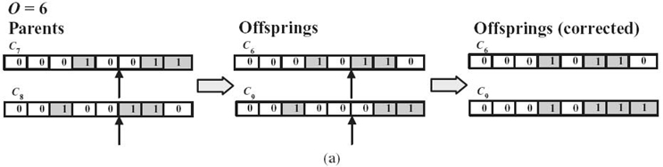
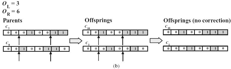
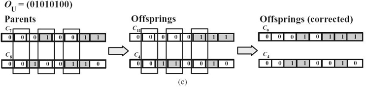
FIGURE 2.7. Illustration of crossover operations: (a) single-point crossover, (b) two-point crossover, and (c) uniform crossover.

Suppose that two parent chromosomes, C₇ = (00010011) and C₈ = (00100110), are selected from the population. By the single-point crossover (shown in Fig. 2.7a), the genes from the crossover point to the end of the two chromosomes exchange with each other to get C₆ = (00010110) and C₉ = (00010111). The crossover point denoted by O = 6 is generated randomly. After crossing, the first offspring, C₆ = (00010110), is a valid solution. However, the other one, C₉ = (00100011), is not valid; thus, we need to perform the correction mechanism. The correction starts from the gene in the position of the crossover point O, that is, g₆. Since g₆ is 1 in the parent chromo-some C₈, it changes to 0 after crossing. We correct it by setting g₆ = 1. Then, C₉ = (00010111) is now a valid solution. In general, we can keep correcting the genes until the end of the chromosome. By the two-point crossover (shown in Fig. 2.7b), the two crossover points are randomly generated, which are O_L = 3 and O_R = 6, and then the genes between O_L and O_R of the two parent chromosomes are exchanged with each other. The two offsprings are C₁₀ = (00100111) and C₁ = (00010010), respectively. Since both of the offspring chromosomes are valid, we do not need to do any correction. As we already know, C₁ is the fittest in the population. This is a good illustration; we can obtain a fitter solution during the evolutionary process through genetic operations. For the uniform crossover (shown in Fig. 2.7c), the vector of uniform crossover O_U is randomly generated, which is O_U = (01010100), indicating that g₂, g₄, and g6 of the two parent chromosomes exchange with each other. Hence, the two offsprings are C₁₁ = (00000111) and C₄ = (00110010). Since C₁₁ is not a valid solution, we need to perform the correction scheme, and the corrected chromosome becomes C₁₀ = (00110010), which is a valid solution.

2.5.6.2   Mutation   The population will undergo the mutation operation after the crossover operation is performed. With a mutation probability P_m, we scan each gene g_i on the parent chromosomes. If the mutation operation needs to be implemented, the value of the gene flips; that is, 0 becomes 1 and 1 becomes 0.

An example is shown in Figure 2.8, assume g₃ is mutated in chromosome C₇. The offspring C₁₁ = (00110011) is a valid solution; thus, no correction is needed. While g₆ and g₈ are mutated in chromosome C₈, the offspring C₁₂ = (001100011) is not a valid solution. Therefore, we perform the similar correction mechanism mentioned in the crossover section to make the offspring C₁₂ valid by correcting g₆ = 1.

2.5.6.3   Replacement Policy   The last step of RMCDS-GA is to create a new population using an appropriate replacement policy. Usually, two chromosomes from the evolution process are utilized to replace the two worst chromosomes in the original population for generating a new population. However, when creating a new population by crossover and mutation, we have a big chance to lose the fittest chromosome. Therefore, an elitism strategy, in which the best chromosome (or a few best chromosomes) is retained in the next generation's population, is used to avoid losing the best candidates.

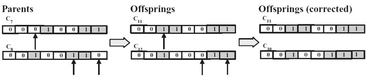
FIGURE 2.8. Illustration of mutation operation.

The RMCDS-GA stops and returns the current fittest solution until the number of total generation G is achieved or the best fitness value does not change for continuous 10 generations. In the RMCDS-GA algorithm, we use G to stop the algorithm.

2.6   PERFORMANCE EVALUATION

In the simulations, we implement the RMCDS-GA to solve the RMCDS problem. These algorithms are compared with Wan's work [14] denoted by MIS, which is the latest and best MIS-based CDS construction algorithm.

2.6.1   Simulation Environment

We build our own simulator where all nodes have the same transmission range (10m) and all nodes are deployed uniformly in a square area. Moreover, a random value between [0.9, 0.98] is assigned to the TSR value associated with a pair of nodes inside the transmission range; otherwise, a random value between (0, 0.8] is assigned to the TSR value associated with a pair of nodes beyond the transmission range. For a certain n, 100 instances are generated. The results are averaged among 100 instances. Additionally, the particular GA rules and control parameters are listed in Table 2.2.

2.6.2   Simulation Results

In Table 2.3, we show that traditional MCDS construction algorithms cannot solve the RMCDS problem under the PNM model, especially for large-scale WSNs. In Table 2.3, we list the number of times that MIS and RMCDS-GA can find a CDS with a reliability greater than or equal to σ by running 100 simulations separately. σ is decreased from 0.6 to 0.4 by 0.1. From Table 2.3, we find that, with increasing n, the numbers of the times of satisfied CDSs for MIS and RMCDS-GA both decrease. This is because the sizes of CDSs increase, which leads to a lower node -to-node delivery ratio. Moreover, RMCDS-GA can guarantee more satisfied CDSs than MIS, especially when n ≥ 200. In other words, for large-scale WSNs, it is hard to construct a satisfied CDS for MIS since the MIS algorithm does not consider reliability. Additionally, both MIS and RMCDS-GA can find more satisfied CDSs when σ decreases. In conclusion, traditional MCDS construction algorithms do not take reliability into consideration, while RMCDS-GA can find a satisfied RMCDS, which is more practical in real environments.

Table 2.2 GA Parameters and Rules

Population size (k)	20
Number of total generations (G)	100
Selection scheme	Roulette wheel selection
Replacement policy	Elitism
Crossover probability (Pc)	1
Mutation probability (Pm)	0.001

TABLE 2.3. MIS -based CDS s and RMCDS-GA-Generated CDS s

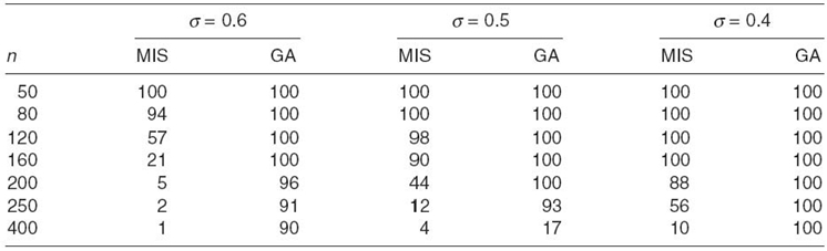
TABLE 2.4. R and | D| Results of MIS and RMCDS-GA Algorithms

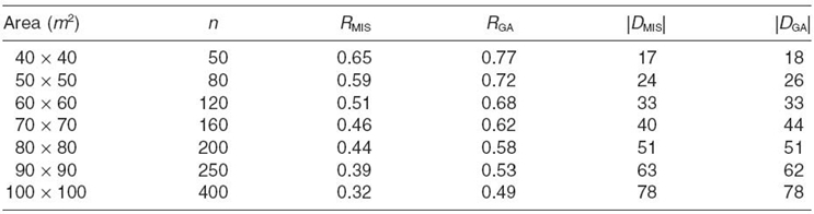
In Table 2.4, R_MIS and R_GA represent the reliability of a CDS generated by MIS and RMCDS-GA, respectively. |D_MIS| and |D_GA| represent the size of the CDS constructed by MIS and RMCDS- GA, respectively. In Table 2.4, the reliability of CDSs decreases when the area size increases since the number of the dominators increases. RMCDS-GA can guarantee to find a more reliable CDS than MIS; that is, R_GA > R_MIS. More importantly, the sizes of the CDSs obtained by MIS and RMCDS-GA are almost the same. On average, RMCDS-GA can find a CDS with 10% more reliability without increasing the size of a CDS than MIS. In summary, RMCDS-GA does not trade CDS size for CDS reliability.

2.7   CONCLUSIONS

In this chapter, we have investigated the RMCDS problem using a new network model called PNM. The PNM model, based on empirical studies, shows that most wireless links are lossy links, which only probabilistically connect pairs of nodes. Different from the traditional DNM model, which assumes that links are either connected or disconnected, the PNM model enables the employment of lossy links by introducing the TSR value on each lossy link. In this chapter, we focus on constructing an MCDS while its reliability satisfies a preset application-dependent threshold. We claim that RMCDS is an NP-hard problem and propose a GA to address the problem. The simulation results show that compared to the traditional MCDS algorithm, RMCDS-GA can find a more reliable CDS without increasing the size of a CDS.

REFERENCES

[1] H. Karl and A. Willig, Protocols and Architectures for Wireless Sensor Networks. Hoboken, NJ: John Wiley & Sons, 2005.

[2] R. Rajaraman, “Topology control and routing in ad hoc networks: A survey,” ACM SIGACT News, 33(2): 60C73, 2002.

[3] W. Di, Q. Yan, and T. Ning, “Connected dominating set based hybrid routing algorithm in ad hoc networks with obstacles,” ICC'06, Turkey, Istanbul, June 11–15, 2006.

[4] E.H. Wassim, A.F. Ala, G. Mohsen, and H.H. Chen, “On efficient network planning and routing in large-scale MANETs,” IEEE Transactions on Vehicular Technology, 58(7): 3796–3801, 2009.

[5] L. Ding, Y. Shao, and M. Li, “On reducing broadcast transmission cost and redundancy in ad hoc wireless networks using directional antennas,” WCNC'08, pp. 2295–2300, 2008.

[6] B.K. Polat, P. Sachdeva, M.H. Ammar, and E.W. Zegura, “Message ferries as generalized dominating sets in intermittently connected mobile networks,” MobiOpp'10, Pisa, Italy, 2010.

[7] A. Helmy, S. Garg, P. Pamu, and N. Nahata, “CARD: A contact–based architecture for resource discovery in ad hoc networks,” Mobile Networks and Applications, 10(1): 99–113, 2004.

[8] B. Deb, S. Bhatnagar, and B. Nath, “Multi–resolution state retrieval in sensor networks,” IWSNPA, 2003.

[9] K.P. Shih, D.J. Deng, R.S. Chang, and H.C. Chen, “On connected target coverage for wireless heterogeneous sensor networks with multiple sensing units,” Sensors, 9(7): 5173‒5200, 2009.

[10] H.M. Ammari and J. Giudici, “On the connected k–coverage problem in heterogeneous sensor nets: The curse of randomness and heterogeneity,” ICDCS, Montreal, Quebec, Canada, 2009.

[11] S. Ji, Y. Li, and X. Jia, “Capacity of dual–radio multi–channel wireless sensor networks for continuous data collection,” INFOCOM, Shanghai, China, April 10– 15, 2011.

[12] S. Ji, Z. Cai, Y. Li, and X. Jia, “Continuous data collection capacity of dual–radio multi–channel wireless sensor networks,” IEEE Transactions on Parallel and Distributed Systems(TPDS), 23(10): 1844–1855, 2011.

[13] S. Ji and Z. Cai, “Distributed data collection and its capacity in asynchronous wireless sensor networks,” Inforcom, Orlando, Florida, March 25–30, 2012.

[14] P.J. Wan, S.C.–H. Huang, L. Wang, Z. Wan, and X. Jia, “Minimum latency aggregation scheduling in multihop wireless networks,” MobiHoc'09, New Orleans, Louisiana, May 18–21, pp. 185–194, 2009.

[15] M. Yan, J. He, S. Ji, and Y. Li, “Minimum latency scheduling for multi–regional query in wireless sensor networks,” IPCCC, Orlando, Florida, USA, November 17–19, 2011.

[16] A. Ephremides, J. Wieselthier, and D. Baker, “A design concept for reliable mobile radio networks with frequency hopping signaling,” Proceedings of the IEEE, 75(1): 56‒73, 1987.

[17] S. Guha and S. Khuller, “Approximation algorithms for connected dominating sets,” Algorithmica, 20: 374–387, 1998.

[18] J. Wu and H. Li, “On calculating connected dominating set for efficient routing in ad hoc wireless networks,” DIALM, pp. 7–14, 1999.

[19] F. Dai and J. Wu, “An extended localized algorithm for connected dominating set formation in ad hoc wireless networks,” TPDS'04, 15(10): 908–920, 2004.

[20] P. Wan, K. Alzoubi, and O. Frieder, “Distributed construction of connected dominating set in wireless ad hoc networks,” Mobile Networks and Applications, 9(2): 141–149, 2004.

[21] M. Cardei, M. Cheng, X. Cheng, and D. Zhu, “Connected dominating set in ad hoc wireless networks,” Proceedings of the 6th International Confrence on Computer Science and Informatics, 2002.

[22] Y. Li, M. Thai, F. Wang, C. Yi, P. Wang, and D. Du, “On greedy construction of connected dominating sets in wireless networks,” Wireless Communications and Mobile Computing, 5(8): 927–932, 2005.

[23] K. Alzoubi, P. Wan, and O. Frieder, “Message-optimal connected dominating sets in mobile ad hoc networks,” MobiHoc'02, pp. 157–164, 2002.

[24] Y. Li, S. Zhu, M. Thai, and D. Du, “Localized construction of connected dominating set in wireless networks,” TAWN, Chicago, June, 2004.

[25] C. Adjih, P. Jacquet, and L. Viennot, “Computing connected dominated sets with multi–point relays,” Ad Hoc & Sensor Wireless Networks, 1(1/2): 27– 39, 2005.

[26] X. Cheng, M. Ding, D. Du, and X. Jia, “Virtual backbone construction in multihop ad hoc wireless networks,” Wireless Communications and Mobile Computing, 6(2): 183–190, 2006.

[27] R. Misra and C. Mandal, “Rotation of CDS via connected domatic partition in ad hoc sensor networks,” TMC, 8(4), 2009.

[28] D. Kim, W. Wang, X. Li, Z. Zhang, and W. Wu, “A new constant factor approximation for computing 3–connected m–dominating sets in homogeneous wireless networks,” INFOCOM, 2010.

[29] L. Ding, X. Gao, W. Wu, W. Lee, X. Zhu, and D.Z. Du, “Distributed construction of connected dominating sets with minimum routing cost in wireless networks,” ICDCS, 2010.

[30] D. Kim, Y. Wu, Y. Li, F. Zou, and D.Z. Du, “Constructing minimum connected dominating sets with bounded diameters in wireless networks,” IEEE Transactions on Parallel and Distributed Systems, 20(2): 147–157, 2009.

[31] J. He, S. Ji, M. Yan, Y. Pan, and Y. Li, “Genetic-algorithm-based construction of load-balanced CDSs in wireless sensor networks,” MILCOM 2011, Baltimore, MD, November 7–10, 2011.

[32] J. He, S. Ji, M. Yan, Y. Pan, and Y. Li, “Load-balanced CDS construction in wireless sensor networks via genetic algorithm,” International Journal of Sensor Networks(IJSNET), 11(3): 166–178, 2011.

[33] J. He, S. Ji, P. Fan, Y. Pan, and Y. Li, “Constructing a load-balanced virtual backbone in wireless sensor networks,” International Conference on Computing, Networking and Communications(ICNC), Maui, HI, January 30–February 2, 2012.

[34] M. Zuniga and B. Krishnamachari, “Analyzing the transitional region in low power wireless links,” SECON, Santa, Clara, October 4–7, 2004.

[35] G. Zhou, T. He, S. Krishnamurthy, and J. Stankovic, “Impact of radio irregularity on wireless sensor networks,” Mobisys, Boston, MA, June 6–9, 2004.

[36] A. Cerpa, J.L. Wong, M. Potkonjak, and D. Estrin, “Temporal properties of low power wireless links: Modeling and implications on multi–hop routing,” MobiHoc, Urbana –Champaign, IL, May 25–28, 2005.

[37] A. Cerpa, J. Wong, L. Kuang, M. Potkonjak, and D. Estrin, “Statistical model of lossy links in wireless sensor networks,” IPSN'05, Los Angeles, CA, 2005.

[38] Y. Liu, Q. Zhang, and L.–M. Ni, “Opportunity–based topology control in wireless sensor networks,” TPDS'10, 21(9), 2010.

[39] M. Al–Obaidy, A. Ayesh, and A. Sheta, “Optimizing the communication distance of an ad hoc wireless sensor networks by genetic algorithms,” Artificial Intelligence, 29: 183–194, 2008.

[40] J. Wang, C. Niu, and R. Shen, “Priority–based target coverage in directional sensor networks using a genetic algorithm,” Computers and Mathematics with Applications, 57: 1915–1922, 2009.

[41] A. Bari, S. Wazed, A. Jaekel, and S. Bandyopadhyay, “A genetic algorithm based approach for energy efficient routing in two–tiered sensor networks,” Ad Hoc Networks, pp. 665–676, 2009.

[42] X. Hu, J. Zhang, Y. Yu, H. Chung, Y. Lim, Y. Shi, and X. Luo, “Hybrid genetic algorithm using a forward encoding scheme for lifetime maximization of wireless sensor networks,” ITEC, 14(5): 766–781, 2010.

[43] A. Agrawal and R. Barlow, “A survey of network reliability and domination theory,” Operations Research, 32: 298–323, 1984.

[44] M.R. Garey and D.S. Johnson, Computers and Intractability: A Guide to the Theory of NP-Completeness. New York: WH Freeman & Co., 1979.

[45] D.E. Goldberg, Genetic Algorithms in Search, Optimization, and Machine Learning. Bel Air, CA: Addison–Wesley Publishing Company, 1989.

[46] S. Lin, J. Zhang, G. Zhou, L. Gu, T. He, and J. Stankovic, “Atpc: Adaptive transmission power control for wireless sensor networks,” Sensys'06, Boulder, CO, October 31–November 3, 2006.

[47] D. Son, B. Krishnamachari, and J. Heidemann, “Experimental study of concurrent transmission in wireless sensor networks,” SenSys'06, Boulder, CO, October 31– November 3, 2006.

[48] J.H. Holland, Adaptation in Natural and Artificial System. Ann Arbor, MI: University of Michigan Press, 1975.

[49] B. Karp and H. Kung, “GPSR: Greedy perimeter stateless routing for wireless networks,” MobiCom '00, New York, 2000.