
17
–––––––––––––––––––––––
Adopting Compression in Wireless Sensor Networks
Xi Deng and Yuanyuan Yang
17.1 INTRODUCTION
Recent years have witnessed the development and proliferation of wireless sensor network (WSNs), attributed to the technological advances of microelectromechanical systems (MEMS) and wireless communications. A WSN is composed of a number of sensor nodes, which are distributed in a specific area to perform certain sensing tasks. A typical sensor node is a low-cost battery-powered device equipped with one or more sensors, a processor, memory, and a short-range wireless transceiver. A variety of sensors, including thermal, optical, magnetic, acoustic, and visual sensors, are used to monitor different properties of the environment. The processor and memory enable the sensor node to perform simple data processing and storing operations. The transceiver makes the sensor node capable of wireless communications, which is critical or WSNs. With many WSNs located in difficult-to-access areas, users usually cannot collect the data in sensor nodes directly. In this case, sensors nodes can transmit the data through the wireless channel to the user or the data sink either directly or by relaying through multiple sensor nodes. Due to the same geographical difficulty, the batteries, as the power supply of the sensor nodes, are difficult to recharge or replace, restricting nodes energy budget. Therefore, energy efficiency is the primary design concern in many WSNs.
Delay-sensitive WSNs are a special type of WSNs that require real-time delivery of sensing data to the data sink. Such networks are widely adopted in various real-time applications including traffic monitoring, hazard detection, and battlefield surveillance, where decisions should be made promptly once the emergent events occur. Thus, delay-sensitive WSNs are more focused on minimizing the communication delay during data delivery rather than the energy efficiency. Recent study in this area has mainly focused on the algorithm design of efficient routing strategies and data aggregation to reduce such delay and to provide real-time delivery guarantees [1–4] In this chapter, we approach this problem from a different and orthogonal angle by considering the effect of data compression. Compression was initially adopted as an effective approach to save energy in WSNs. In fact, it can also be used to reduce the communication delay in delay-sensitive WSNs.
In WSNs, compression reduces the data amount by exploiting the redundancy resided in sensing data. The reduction can be measured by the compression ratio, defined as the original data size divided by the compressed data size. A higher compression ratio indicates larger reduction on the data amount and results in shorter communication delay. Thus, much work in the literature has been endeavored to achieve better compression ratio for sensing data. However, from the implementation perspective, most of the compression algorithms are complex and time-consuming procedures running on sensor nodes which are very resource constrained. As the processing time of compression could not be simply neglected in such nodes, the effect of compression on the total delay during data delivery becomes a trade-off between the reduced communication delay and the increased processing time. As a result, compression may increase rather than decrease the total delay when the processing time is relatively long.
We first analyze the compression effect in a typical data gathering scheme in WSNs where each sensor collects data continuously and delivers all the packets to a data sink. To do so, we need to first obtain the processing time of compression, which depends on several factors, including the compression algorithm, processor architecture, CPU frequency, and the compression data. Among numerous compression algorithms, we use the Lempel–Ziv–Welch (LZW) [5] as an example, which is lossless compression algorithm suitable for sensor nodes. We implement the algorithm on a TI MSP430F5418 microcontroller (MCU) [6], which is used in the current generation of sensor nodes. Experiments reveal that the compression time in such a system is comparable to the transmission time of packets and thus cannot be simply ignored. To support the study in large-scale WSNs, we utilize software estimation approach to providing runtime measurement of the algorithm execution time in the network simulation. The simulation results show that compression may lead to several times longer overall delay under light traffic loads, while it can significantly reduce the delay under heavy traffic loads and increase maximum throughput.
Since the effect of compression varies heavily with network traffic and hardware configurations, we give an online adaptive algorithm that dynamically makes compression decisions to accommodate the changing state of WSNs. In the algorithm, we adopt a queueing model to estimate the queueing behavior of sensors with the assistance of only local information of each sensor node. Based on the queueing model, the algorithm predicts the compression effect on the average packet delay and performs compression only when it can reduce packet delay. The simulation results show that the adaptive algorithm can make decisions properly and yield near-optimal performance under various network configurations.
17.2 COMPRESSION IN SENSOR NODES
Due to the limited energy budget in sensor networks, compression is considered as an effective method to reduce energy consumption on communications and has been extensively studied. In the meanwhile, the spatial-temporal correlation in the sensing data makes it suitable for compression. Akyildiz et al. proposed a theoretical framework to model the correlation and its utilization in several possible ways [7]. Scaglione and Servetto proved that the optimal compression efficiency can be achieved by source coding with proper routing algorithms [8]. The relationship between compression and hierarchical routing was also discussed in Reference 9. Pattem et al. analyzed the bound on the compression ratio achieved by lossless compression and showed that a simple, static cluster-based system design can perform as well as sophisticated adaptive schemes for joint routing and compression [10]. In Reference 11, framework of distributed source coding (DSC) was given to compress correlated data without explicit communications. However, the implementation of DSC in practice could be difficult as it requires the global knowledge of the sensor data correlation structure.
Compression algorithms for sensor nodes can be classified into lossy compression and lossless compression. Lossy compression is defined in the sense that the compressed data may not be fully recovered by decompression. series of algorithms utilized the data correlation to reduce the amount of data to be gathered while keeping the data within an affordable level of distortion. The approaches include data aggregation [12, 13], where only summarized data are required, approximate data representation using polynomial regression [14], line segment approximation [15], and low-complexity video compression [16].
Lossless compression can reconstruct the original data from the compressed data. Coding by ordering [17] is compression strategy that utilizes the order of packets to represent the values in the suppressed packets. PINCO [18] was proposed to compress the sensing data by sharing the common suffix for the data. This approach is more useful for data with sufficiently long common suffices, such as node ID and time stamp. In Reference 19, the implementation of the LZW compression algorithm in sensor nodes was extensively studied and showed to have a good compression ratio for different types of sensing data. Another compression algorithm, Squeeze.KOM [20], uses stream-oriented approach that transmits the difference, rather than the data itself, to shorten the transmission. Interested readers can also find survey on compression algorithms in Reference 21.
Here we use the LZW algorithm as an example to evaluate its compression effects. Compared to other compression algorithms, LZW is relatively simple but yields good compression ratio for sensor data as shown in Reference 19 Next, we briefly introduce the LZW algorithm and the approach to obtain its execution time at the software level instead of running the algorithm on hardware.
17.2.1 LZW Algorithm
LZW compression is dictionary-based algorithm that replaces strings of characters with single codes in the dictionary. The first 256 codes in the dictionary by default correspond to the standard character set. As shown in Table 17.1, the algorithm sequentially reads in characters and finds the longest string s that can be recognized by the dictionary. Then, it encodes s using the corresponding code word in the dictionary and adds string s + c in the dictionary, where c is the character following string s This process continues until all characters are encoded. more detailed description of the LZW algorithm can be found in Reference 5.
TABLE 17.1. Compression Algorithm
| STRING = first character |
| while there are still input chacters |
| C = next character |
| look up STRING + C in the dictionary |
| STRING = STRING + C |
| else |
| output the code for STRING |
| add STRING + C to the dictionary |
| STRING = C |
| else if |
| end while |
| output the code for STRING |
We consider only the compression process but not the decompression process because the latter can be finished in relatively short time when it is performed at the sink node with more powerful computation capability. To adapt the LZW compression to sensor nodes, we set the dictionary size to 512, which has been shown to yield good compression ratios in real-world deployments [19].
To achieve a good compression ratio, which is the ratio of the original data size to the compressed data size, the string should be long enough to provide sufficient redundancies. Thus, the LZW algorithm is more suitable for WSNs that collect heavier load data, such as images and audio clips. Even in the compression algorithms specifically designed for this type of data, the processing in the algorithms could be complex and time-consuming. Hence, the evaluation result on the LZW algorithm can provide guidance for adopting these algorithms. In addition, in large-scale WSNs, distant nodes require multiple hops of transmissions to reach the sink, and the nodes closer to the sink may endure unaffordable traffic. In this case, aggregation is often used (e.g., in cluster-based networks) to reduce the traffic, and such aggregated packets consisting of several lighter load packets are also suitable for compression.
17.2.2 Compression Delay in Sensor Nodes
We examine the compression process on a TI MSP430F5418 MCU, which is used in the current generation of sensor nodes. It is a 16-bit ultra-low-power MCU with 128-kB flash and 16-kB RAM. The CPU has a peak working frequency of 18 MHz, a very high frequency among the current generation of sensor nodes.
To facilitate the evaluation of the compression effect in large-scale WSNs, we adopt a software estimation approach to simulate the compression processing time. Since instructions are sequentially executed in the CPU of this MCU, the processing time can be calculated as the total number of instruction cycles divided by the CPU frequency. Thus, obtaining the precise cycle counts becomes the main task, which we describe below.
TABLE 17.2. A Mapping Example for Function in the LZW Algorithm
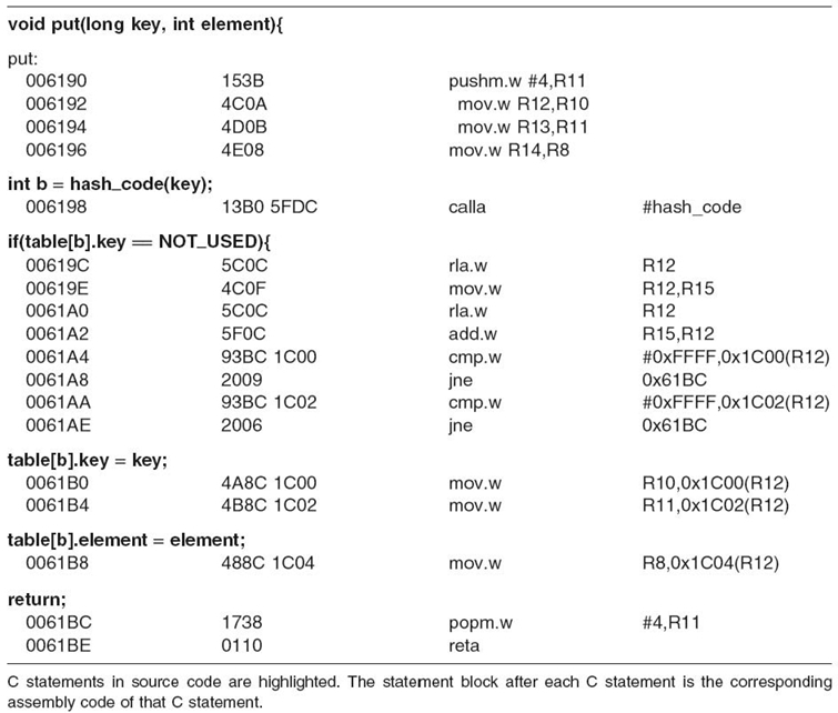
The source code of the LZW algorithm written in language is first compiled to assembly code using the instruction set of the MSP430X CPU series. A mapping is performed between the source code and the corresponding assembly code, with an example shown in Table 17.2. As each instruction in assembly code has a fixed number of execution cycles, the number of cycles of each statement can be counted by summing up the numbers of cycles of the corresponding assembly instructions. The numbers for all statements are then recorded in the source code by code instrumentation so that the execution cycles can be obtained at runtime. For the efficiency consideration, the instrumentation codes only appear at the end of each basic block, in which statements are sequentially executed without conditional branches. This way, the total count of cycles can be obtained at the completion of the LZW algorithm, then the processing time is obtained by dividing the total execution cycles by the working frequency.
17.3 COMPRESSION EFFECT ON PACKET DELAY
In this section, we study the compression effect on packet delay for data gathering in WSNs. We consider the all-to-one data gathering scenario where all sensors continuously generate packets and deliver them to a single sink. The performance metric used is the end-to-end packet delay, which is the interval from the time a packet is generated at the source to the time the packet is delivered to the sink. To evaluate the compression effect, we compare the end-to-end packet delay with compression and without compression. In the rest of this chapter, we refer to these two schemes as compression scheme and no-compression scheme, respectively.
17.3.1 Experiment Setup
The experiments are conducted in the NS-2 simulator, a widely used network simulator. To simplify the evaluation, we examine the performance on a two-dimensional (2-D) grid wireless network. Two networks of a 5 × 5 grid and a 7 × 7 grid with the sink at the center of the grids are considered. In the simulation, the transmission range is set to 16 m and the distance between neighboring nodes is 10 and 15 m, respectively, to create different network topologies. The packet generation on each sensor node follows an i.i.d. Poisson process, and we assume an identical packet length for all the packets generated in a single experiment. Two different packet lengths (256 and 512 B) are used to create different compression ratios and processing delays.
At the network layer, we a adopt multipath routing strategy [22] Specifically, each sensor is assigned a level number, which indicates the minimum number of hops required to deliver a packet from this sensor to the sink. Such information can be obtained at the initial setup in the sensor deployment. A sensor with a level number i is called a level i node. A level i node only forwards the packets to its level i − 1 neighbors. Such a routing strategy is easy to implement but may not necessarily yield the best real-time performance. However, since the compression strategy adopted does not consider interpacket compression, the choice of the routing strategy will not substantially affect the performance evaluation that targets at the compression algorithm.
As we aim at delay-sensitive networks where packet delay rather than energy efficiency is the primary concern, we adopt the commonly used 802.11 protocol as the medium access control (MAC) layer protocol, and the wireless bandwidth is set to 1 Mb/s. The data set is automatically generated by the tool described in Reference 23, which provides a good approximation on the real sensing data in the evaluation of several representative network applications. We use such synthetic data so that the simulation can be performed sufficiently long to capture the steady-state behavior without exhausting the simulation data.
Compression is performed on each packet when it is generated at the source node. Since each sensor is equipped with a sequential processor, multiple packets are served in the first-come-first-served order and sufficiently large buffer is assumed so that no packets are dropped at the compression stage. The compression process is simulated according to the estimation approach described in Section 17.2. The CPU frequency is 18 MHz. With these settings, we obtain that the average compression ratio is 1.25 and 1.6 when the packet length is 256 and 512 B, respectively. The average processing delay is 0.016 second for 256-B packets and 0.045 second for 512-B packets. The delays are further compared with the measurements on the real hardware, and the simulation accuracy is over 95%. Besides, the processing delay could be increased if lower CPU frequencies or more complex compression algorithms are adopted. For example, it is suggested that the Burrows‒Wheeler transform (BWT) [24] can be performed on the sensor data to assist the subsequent LZW compression to obtain better compression ratio. Such processing delay can greatly affect the performance of high-resolution mission-critical applications, including real-time multimedia surveillance and other applications with time-liness requirement, where the extra delay could be critical for some packets to meet their deadlines.
17.3.2 Experimental Results
Based on the routing strategy, a packet generated at a level i node requires i-hop transmissions to reach the sink, resulting in different packet delays for nodes at different levels. In this section, we examine the average packet delay for all the nodes at the same level. Figure 17.1 shows the average delays of different levels in the 5 × 5 network with the neighboring distance set to 15 m and the packet length set to 512 B.
The primary observation drawn from the figure is that compression has a two-sided effect on the real-time performance depending on the packet generation rate. When the rate is low, compression clearly increases the average delay at each level. For example, when the rate is 2, the average delay of level is increased by about 2.7 times from 13.6 to 51.5 ms when compression is adopted. Such increase is also observed for other levels, the least of which is 75% for level 4. Note that under such light traffic load, the delay is almost the packet transmission time due to little contention for the wireless channel. Since the packet transmission time reduced by compression is much less than the increase caused by the compression processing time, the overall delay increases, indicating a negative effect of compression. We also notice that such increase is smaller for nodes at higher levels, which can be explained by the fact that nodes at higher levels require more hops of transmissions to reach the sink, while each transmission is shortened due to the compression. Hence, their delay increase caused by compression processing becomes a smaller portion in the total packet delay.
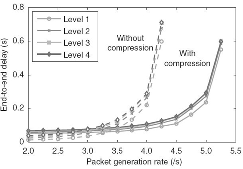
FIGURE 17.1. Average packet delays for packets generated at different levels.
On the other hand, when the packet generation rate becomes higher, the average delays in both schemes increase and the increase in the no-compression scheme grows much faster than that in the compression scheme. When the rate is higher than 3.5, the compression effect becomes positive and yields significant reduction on average delay. In this case, the traffic in the no-compression scheme becomes heavy and the wireless channel is approaching saturation. Consequently, the packet transmission time and the waiting delay grow rapidly due to channel contentions. On the other hand, compression shortens the packet length and the transmission time, thus effectively reducing the channel utilization and the packet delay, which explains the much slower growth of the packet delay with compression.
Another observation we can draw is that the delays of different levels are quite similar. It implies that the main effect of compression is on the transmissions from level nodes to the sink. This is due to the fact that level nodes undergo the heaviest traffic and hence the longest transmission delay. In this case, compression can achieve much more benefit for the transmissions of level nodes than those nodes at higher levels. Thus, based on this observation, it is reasonable to use the average delay among all the nodes in the network to approximate the delays of nodes at different levels. Figure 17.2 thus shows the average end-to-end delay with different network configurations. We can see that the results reveal similar trend on the end-to-end delay for different network configurations.
To further examine the details of compression effect, we define two rates: maximum packet generation rate and threshold rate The maximum packet generation rate is the rate at which the wireless channel approaches saturation. Technically, we define it as the maximum rate at which the packet delay is smaller than second. The threshold rate is the generation rate at which the packet delay remains unchanged in both no-compression and compression schemes. When the packet generation rate is between the threshold rate and the maximum generation rate, compression reduces the end-to-end delay, showing a positive effect. Otherwise, it increases the packet delay, showing a negative effect. Figure 17.3 shows the relationship between the threshold rates and the maximum generation rates in the compression scheme under different network configurations. We can see that the maximum generation rate and the threshold rate vary a lot with different network configurations. Intuitively, compression should be performed only when the packet generation rate is higher than the threshold rate. However, as shown in the figure, the threshold rate cannot be obtained in advance. Therefore, it is necessary to design an online adaptive algorithm to determine when to perform compression on incoming packets at each node.
17.4 ONLINE ADAPTIVE COMPRESSION ALGORITHM
In this section, we introduce an online adaptive compression algorithm that can be easily implemented in sensor nodes to assist the original LZW compression algorithm. The goal is to accurately predict the difference of average end-to-end delay with and without compression by analyzing the local information at a sensor node and to make right decisions on whether to perform packet compression at the node. The adaptive algorithm is implemented on each sensor node as adaptive compression service (ACS) in an individual layer created in the network stack to minimize the modification of existing network layers. Next, we first introduce the architecture of ACS and then describe the algorithm in detail.
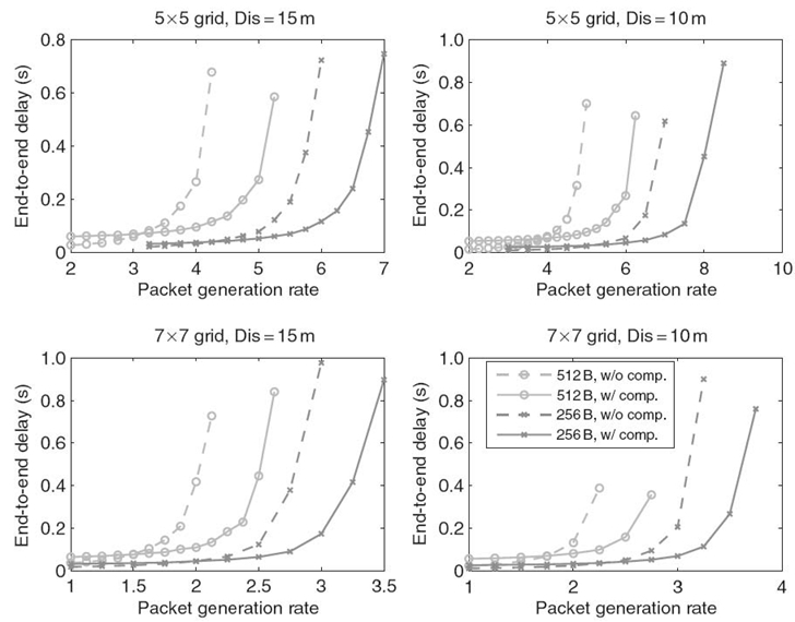
FIGURE 17.2. Average packet delays under various configurations, where d represents the neighboring distance.
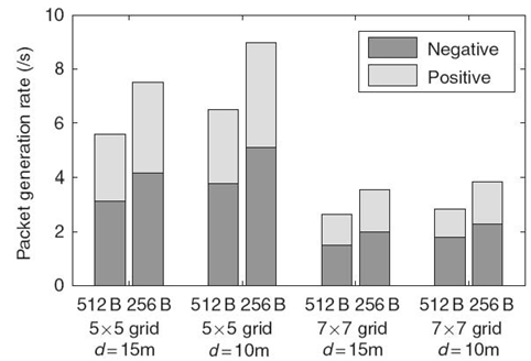
FIGURE 17.3 Different threshold rates under various confi gurations, where d represents the neighboring distance. The compression effect at the threshold rate is neither positive nor negative.
17.4.1 Architecture of ACS
The architecture of ACS is described in Figure 17.4. Located between the MAC layer and its upper layer, ACS consists of four functional units: a controller, an LZW compressor, an information collector, and a packet buffer. The controller manages the traffic flow and makes compression decisions on each incoming packet in this layer. The LZW compressor is the functional unit that performs the actual packet compression by the LZW algorithm. The information collector is responsible for collecting local statistics information about the current network and hardware conditions. The packet buffer is used to temporarily store the packets to be compressed.
With ACS, the traffic between the MAC layer and the upper layer is now intervened by the controller in ACS. All outgoing packets coming down from the upper layer are received by the controller, which maintains two states. In the no-compression state, all packets are directed to the MAC layer without further processing; in the compression state, only compressed packets, which are received from other nodes, will be directly sent down to the MAC layer, and other packets are sent to the packet buffer for compression. On the other hand, for incoming packets from the MAC layer, only the arrival time is recorded by the collector and the packets themselves are sent to the network layer without delays.
Since compression is managed by the node state, the function of the adaptive algorithm is to determine the node state according to the network and hardware conditions. In the adaptive algorithm, we utilize a queueing model to estimate current conditions based on only local information of sensor nodes. In the next section, we introduce the queueing model.
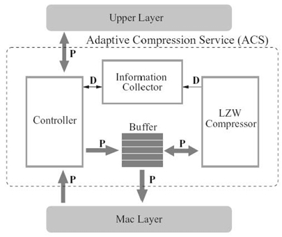
FIGURE 17.4. Architecture of ACS, which resides in a created layer between the MAC layer and its upper layer. P, packet; D, statistics data.
17.4.2 Queueing Model for a WSN
The queueing model for a WSN includes both the network model and the MAC model, which defines the network topology, traffic model, and MAC layer protocol. For a clear presentation, we list the notations that will be used in the model in Table 17.3.
| N | Number of sensor nodes in the WSN |
| R | Radius of the circular region, also the number of levels |
| ni | Number of nodes in level i |
| λg | Packet generation rate |
| λe | Arrival rate of external packets from neighbors |
| pkj | Transitions probability, the probability tha a packet is served by node k and transferred to node j |
| λi | Mean arrival rate for nodes in level i |
| Ttrans | The minimum time of a successful transmission |
| Ldata | Length of the data packet |
| Tctl | Sum of length of all control packets in a transmission |
| nsus | Number of suspensions in the backoff stage |
| cmac | Coeffi cient of variance (COV) of the MAC layer service time |
| Average packet waiting time of the queue | |
| λ | Arrial rate of the queue |
| P | Utilization of the queue |
| cA | COV of the interarrival time |
| cB | COV of the service time |
| rc | Average compression ratio |
| Tp | Average compression processing ttime |
| cp | COV of the processing time |
| pc | Ratio of compressed packet waiting time at the compression queue |
| ΔTmac(i) | Delay reduction in level i |
| ΔTmin | Lower bound of total delay reduction |
17.4.2.1 Network Model: Topology and Traffic We consider a WSN where N sensor nodes are randomly distributed in a finite 2-D region. For calculation convenience, we consider a region of a circular shape with radius R (As will be seen in the experimental results, when the region shape changes, it will not substantially affect the performance of the algorithm.) Every node has an equal transmission range r A data sink is located at the center of the circular region, and all sensor nodes send the collected data to the sink via the aforementioned multipath routing strategy.
If the node density is sufficiently high, we can assume that each node can always find a neighbor whose distance to the sink is shorter than its own distance to the sink by r Thus, nodes between two circles with radius (i − 1)·r and i·r can deliver packets to the sink with i transmissions. According to the routing strategy, these nodes are considered level i nodes. Without loss of generality, we assume r = 1, and there are a total of R levels of nodes. Denote the number of nodes at level i as ni. Then, the average number of nodes at level i can be calculated by
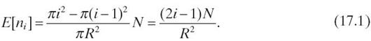
Such a network can then be represented by an open queueing network where each sensor node is modeled as a queue with an external arrival rate λg, which corresponds to the packet generation rate. Denote λji as the arrival rate of node j at level i When i < R, by queueing theory, we have
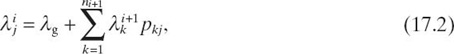
where pkj is the transition probability from node k at level i + 1 to node
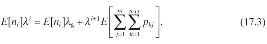
![]() , the above equation can be written as
, the above equation can be written as
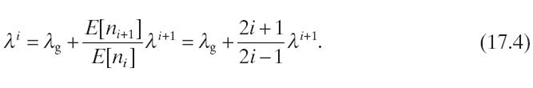
Thus, each node can estimate the arrival rates of nodes at other levels based on its own arrival rate. To evaluate the performance of the queueing system, we also need another important parameter, the average packet service time, which includes the possible packet compression time and the MAC layer service time. While the compression time can be obtained directly from the LZW algorithm, the calculation of the MAC layer service time requires an understanding of the MAC model.
17.4.2.2 MAC Model The MAC layer packet service time is measured from the time when the packet enters the MAC layer to the time when the packet is successfully transmitted or discarded due to transmission failure. To analyze the packet service time, we first briefly describe the distributed coordination function (DCF) of IEEE 802.11 [25] used as the MAC layer protocol.
DCF employs a backoff mechanism to avoid potential contentions for the wireless channel. To transmit a packet, a node must conduct a backoff procedure by starting the backoff timer with a count-down time interval, which is randomly selected between [0, CW) where CW is the contention window size. The timer is decremented by 1 in each time slot when the channel is idle and is suspended upon the sensing of an ongoing transmission. The suspension will continue until the channel becomes idle again. When the timer reaches zero, the node completes the backoff procedure and starts transmission. The entire procedure is completed if the transmission is successfully acknowledged by the receiver. Otherwise, the transmission is considered failed, which invokes a retransmission by restarting the backoff timer. In each retransmission, the contention window size CW will be doubled until it reaches the upper bound defined in DCF. Finally, the packet will be discarded if the number of retransmissions reaches the predefined limit.
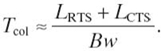
In the MAC layer, we also adopt the request to send (RTS)/clear to send (CTS) mechanism to reduce transmission collisions. Thus, it requires at least four transmissions to successfully transmit a data packet: the transmissions of RTS, CTS, data, and acknowledgment (ACK) packets. Let Ttran denote the minimum packet transmission time, which can be calculated as the sum of all packet lengths divided by network bandwidth Bw
where Lctl = LRTS + LCTS + Lhdr + LACK and Lhdr is the header size of the data packet. Let Tsus denote the average duration of the timer suspension in the backoff stage and Tcol denote the average time spent in transmission collisions. The suspension duration is actually the time waiting for other nodes to complete a packet transmission. Under the assumption of the constant packet length, we can approximately have Tsus = Ttran. On the other hand, with the RTS/CTS mechanism, the collision mainly occurs during the transmission of RTS and continues until the timeout for CTS. Hence,
The overall MAC layer packet service time can then be calculated as
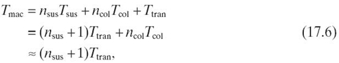
where nsus represents the number of suspensions and ncol is the number of transmission collisions. The last step approximation in Equation (17.6) is due to the relatively small value of both ncol and Tcol. We also exclude the backoff time and some interframe spaces in the above equation due to the same reason.
17.4.2.3 Queueing Analysis for a Sensor Node The queueing model of a sensor node is different in different node states. In the no-compression state, each node is considered as a single queue. Its arrival process is combination of the local packet generation process and the departure processes of its neighbors that send packets to the node. As the simulation results in Reference 26 showed, the departure process of nodes adopting IEEE 802.11 MAC protocol can be approximated as a Poisson process. Thus, we assume that the arrival process of each node is Poisson process and each node is an M/G/1 (i.e., exponential interarrival time distribution/general service time distribution/a single server) queue. In the compression state, the queueing model of each node can be modified as a system of two queues as shown in Figure 17.5 with the compression queue and the transmission queue corresponding to ACS and the MAC layer, respectively. The compression queue can be modeled as an M/G/1 queue because its arrival process, as a split of the arrival process of the sensor node, can also be considered as a Poisson process. On the other hand, since its departure process, a part of the arrival process of the transmission queue, is not a Poissonian, we model the transmission queue as a GI/G/1 queue where GI represents the general independent interarrival time distribution.
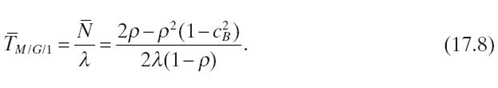
For the M/G/1 queue, according to the well-known Pollaczek–Khinchin formula, the average number of packets N in an M/G/1 queue can be calculated as
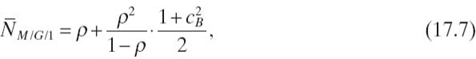
where ρ is the utilization of the queue and cB is the coefficient of variance (COV) of the service time. By Little s law, given the arrival rate λ, the average packet waiting time, which is the packet delay in the node, can be derived as
To derive the average packet waiting time for the transmission queue, we use the diffusion approximation method [27], which is briefly introduced here. Consider an open GI/G/1 queueing network with n nodes. Given the arrival rate λk for node k, k ∈ [1, n], the COV of the interarrival time at node j, cAj, can be approximated as
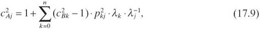
where cBk represents the COV of the service time at node k and cB0 represents the COV of the external interarrival time. In Figure 17.5, we assume the COV of the service time at the compression queue is cp and the portion of compressed packets in all packets is pc. Then, we obtain the COV of the service time at the transmission queue as
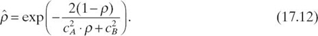
The average packet waiting time can then be approximated by
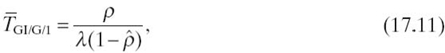
where
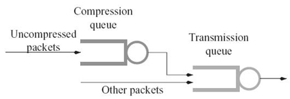
. FIGURE 17.5 Queueing model of a sensor node with compression.
17.4.3 Adaptive Compression Algorithm
We are now in the position to describe the adaptive compression algorithm, which can be divided into two stages: information collection and node state determination.
17.4.3.1 Information Collection In ACS, the information collector is responsible for collecting three types of statistics information:
- Compression statistics, including the average compression ratio rc, the average compression processing time Tp, and the COV of the processing time cp. Upon each packet compression, the compression ratio, the processing time, and its square are recorded. The statistics is updated after every m packet is compressed. In the experiments, we set m = 100. Since the compression statistics can only be collected when nodes perform compression, the network should include an initial phase when all nodes perform compression to obtain the initial values. We assume the sensing data has a stable distribution so that the collecting method above is sufficient to provide proper statistics.
- Packet arrival rates, which include the arrival rate of external packets from neighbors λe and the packet generation rate λg The calculations follow a time-slotted fashion. In each time slot, the total number of packets arrived is counted and the arrival rates are calculated by dividing the total counts by time. Noting that not all external packets are compressed in the adaptive algorithm, we also record the ratio of compressed packets in the external packets as pc.
- MAC layer service time. Since the MAC layer service is considered as an arbitrary process in the queueing model, its mean Tmac and COV cmac are calculated and recorded for the subsequent analysis. The calculation is done along with the calculation of arrival rates in the same time slot to reduce the implementation complexity.
17.4.3.2 State Determination In ACS, the controller determines the appropriate node state according to the statistics information collected. Since most of the information is collected in a time-slotted manner, the decision on the node state is made at the end of each time slot. Depending on the current node state, the decision process is slightly different. Thus, we first consider the case when the node is currently in the no-compression state. Then, the task of the controller is to decide whether performing compression on this node can reduce packet delays. From the experimental results in Section 17.3, we know that compression introduces an extra delay due to compression processing and reduces the packet delay from the current node to the sink. We now discuss these two delays separately.
The incoming packets of the compression queue are the uncompressed portion of the arrival packets at the node. With the information provided by the collector, the arrival rate can be calculated by λc = λ e (1 − pc) + λg, while the service rate is 1/Tp, and the utilization equals λcTp By Equation (17.8), the increased compression time for a packet can be derived as

As the ultimate goal of compression is to reduce the average delay, which is equivalent to reducing the sum of delays of all packets, we define normalized delay as the total delay for all packets in a unit time. Thus, for a time interval t, the total increased delay due to compression is λctTcom, and the normalized delay increase is λcTcom
Now let us look at the delay reduction in packet delivery after compression. While it is difficult to accurately calculate this reduction, we can easily obtain a lower bound. Given the compression ratio rc and the length of the original packet L, the packet length is shortened by L − Lrc after compression and its transmission time is reduced by at least
![]()
For a level i node, there are i transmissions for this packet after compression. Thus, the total reduction is at least
![]()
We compare this lower bound with the increased compression time Tcom. If Tcom ≤ Δ Tmin, the node is switched to the compression state.
When Tcom > ΔTmin, we need to calculate the normalized delay reduction. In fact, if only one node performs compression, there will be no extra reduction other than the reduced transmission time because the surrounding traffic will not change. However, according to the network model, nodes at the same level should share very similar traffic conditions; thus, although made independently, their state determination is likely to coincide. Therefore, when we consider the delay reduction due to compression on a node, it is reasonable to assume that other nodes at the same level will also perform compression. In this sense, compression actually affects the transmissions of all packets in the node rather than only the uncompressed packets. Furthermore, such effect not only resides in the local node but also in the downstream nodes on the routing path when they receive those compressed packets. Thus, we need to examine the delay reduction level by level.
We first examine the delay reduction in the local node. Without loss of generality, we assume the node is at level i The packet delay before compression can be obtained by Equation (17.8), where λ = λg + λe, ρ = λTmac, and cB = cmac. When compression is performed, the transmission queue is modeled as a GI/G/1 queue and the packet delay is calculated by Equations (17.11) and (17.12). According to Figure 17.5, the arrival rate of the transmission queue does not change after the compression. cA can be calculated by Equation (17.10) and cB is approximated to be cmac. Next, we derive the average service time after compression from Tmac. Based on the analysis in Section 17.4.2, the service time Tmac is approximately proportional to the packet transmission time Ttran and hence Ldata + Lctl. We assume the original packet length is L and the compressed packet length is then L/rc, where rc is the compression ratio obtained in the collector. Thus, Ldata is reduced from L − pc (L − L/rc) to Lrc by compression, while Lctl keeps unchanged. The average service time after compression can then be calculated as
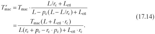
With all these parameters known, the packet delay after compression can be obtained and so is the delay reduction, denoted as Tmac(i).
Now we estimate the delay reduction at a level k node (k < i) on the routing path. According to the analysis in Section 17.3, higher-level nodes enjoy more compression benefit through the transmissions on longer routes, indicating that they tend to perform compression more aggressively. Given the local node in the no-compression state, it is reasonable to assume that the nodes with the same packet generation rates at level k are also in the no-compression state. Then, the packet delay at this node is calculated with Equation (17.8). By Equation (17.4), we can derive the arrival rate by λg and λe. The calculation of the service time Tmac mainly depends on the value of nsus and Ttran. While Ttran can be calculated in a similar way as for the local node, nsus cannot be derived intuitively. In Reference 28, it was shown that nsus is proportional to the utilization ρ if ρ is shared by all nodes in its interfering range. For the network under consideration, we approximately assume that nodes in the interfering range of a level k node are all in level k. Then, we have
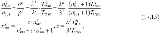
where parameters for the level i and k nodes are labeled with the superscript i and k, respectively. With nsus and Ttran obtained, the service time can be obtained and so is the reduction, which we denote as Tmac (k).
The normalized delay reduction can be calculated as
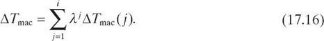
The decision on the state of the node is then made by comparing Tmac with λc Tcom. The procedure of the state determination in pseudocode is given Table 17.4.
When the node is currently in the compression state, all the calculations will also be performed. The only difference is that we compare the reduced processing time with the increased transmission time due to compression cancellation.
TABLE 17.4. State Determination Procedure, Performed at the End of Each Time Slot for a Node in the No-Compression State
| For each node at level i: |
| if state = No-Compression then |
| read statistics from the information collector |
| compute Tcom and Tmin |
| if Tcom≤ΔTmin |
| set state to Compression |
| else |
| set i to the node s level number |
| set Tmac to zero |
| while i > 0 |
| Calculate λi |
| compute reduction ΔTmac (i) |
| add λiΔTmac (i) to ΔTmac |
| decrease i by one |
| end while |
| ifλcTcom ≤ ΔTmacthen |
| set state to Compression |
| end if |
| end if |
| end if |
17.5 PERFORMANCE EVALUATIONS
With the online adaptive compression algorithm, each node can dynamically decide whether a packet is compressed or not, adapting to the current network and hardware environment. In this section, we present the performance evaluation results for the adaptive compression algorithm. We compare the performance of the adaptive scheme with other two schemes: the no-compression scheme, in which no packets are compressed at all, and the compression scheme, where all packets are compressed in data gathering.
The experiments are conducted in three networks: a 7 × 7 grid, a 9 × 9 grid, and a 11 × 11 grid. The sink is located at the center of the grid. The transmission range is 1.5 times of the neighboring distance. The original packet length is set to 512 B. Other parameters are similar to the configuration in the previous experiments in Section 17.3.
In the simulation, the packet generation rate starts at a rate lower than the threshold rate and then increases linearly every 300 seconds. Such increase continues until the maximum rate is reached, at which time the simulation also ends. The time slot length used in the information collector is 30 seconds. Figure 17.6 shows the average end-to-end delays for three schemes in different networks. We can see that the delay for the adaptive scheme is always close to the lower one of the no-compression and compression schemes, indicating overall good adaptiveness of the algorithm on the network traffic. In particular, when the generation rate is lower than the threshold rate, the adaptive scheme chooses not to compress packets and thus yields nearly the same results as the no-compression scheme. When the generation rate is slightly higher than the threshold, the adaptive scheme yields similar results as the compression scheme except some points with slightly longer delays in the 9 × 9 grid and the 11 × 11 grid. The largest increase in delay is only 10% when the generation rate is 0.9 in the 11 × 11 grid. Such consistently good performance in different networks indicates a good scalability of the algorithm on the network size.
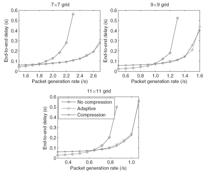
FIGURE 17.6. The overall average packet delays under three schemes in three different networks.
We further examine the delays for different levels to provide a comprehensive illustration. Figure 17.7 depicts the average delays for different levels in the 9 × 9 grid network. It can be noticed that, for nodes at level 1, the adaptive scheme outperforms other two schemes when the generation rate exceeds the threshold rate. For nodes at levels and at the same generation rate, however, the average delays under the adaptive scheme are slightly longer than that under the compression scheme. This can be explained by the observation that the threshold rates for higher-level nodes are lower than the thresholds for lower-level nodes. When the generation rate is between two different threshold rates, higher-level nodes perform compression, while the lower-level nodes do not. Therefore, without suffering from the compression processing delay, lower-level nodes can still enjoy the benefit of the reduced average packet length as they receive packets from higher-level nodes, resulting in shorter delays than that under the compression scheme. On the other hand, since lower-level nodes do not perform compression, the average packet length and the subsequent transmission delay become longer, increasing the end-to-end delay for other nodes. Such increase is also more evident for higher-level nodes as the generated packets in these nodes endure more hops of prolonged transmissions during the delivery to the sink.
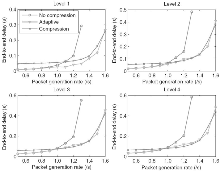
FIGURE 17.7. The average delays for packets generated at different levels under three schemes in 9 × 9 grid network.
17.6 SUMMARY
In this chapter, we have discussed the effect of the compression on end-to-end packet delay in data gathering in WSNs. To accurately examine the effect of compression, we incorporate the hardware processing time of compression in the experiments by utilizing a software estimation approach to measuring the execution time of a lossless compression algorithm, LZW, on TI MSP430F5418 MCU. Through simulations, we have found that compression has a two-sided effect on packet delay in data gathering. While compression increases the maximum achievable throughput, it tends to increase the packet delay under light traffic loads and to reduce the packet delay under heavy traffic loads. We also evaluate the impact of different network settings on the effect of compression, providing a guideline for choosing appropriate compression parameters.
We then describe an online adaptive compression algorithm to make compression decisions based on the current network and hardware conditions. The adaptive algorithm runs in a completely distributed manner. Based on a queueing model, the algorithm utilizes local information to estimate the overall network condition and switches the node state between compression and no-compression according to the potential benefit of compression. The experimental results show that the adaptive algorithm can fully exploit the benefit of compression while avoiding the potential hazard of compression. Finally, it should be pointed out that this adaptive algorithm is not restricted to the LZW compression algorithm, and in fact, it can be applied to any practical compression algorithms by simply replacing the compressor in ACS.
REFERENCES
[1] T. He, J.A. Stankovic, C. Lu, and T. Abdelzaher, “SPEED: A stateless protocol for real-time communication in sensor networks,” in Proceedings of the IEEE ICDCS, 2003.
[2] E. Felemban, C. Lee, and E. Ekici, “MMSPEED: Multipath multi-SPEED protocol for qos guarantee of reliability and timeliness in wireless sensor networks,” IEEE Transactions on Mobile Computing, (6): 738‒754, 2006.
[3] T. He, B.M. Blum, J.A. Stankovic, and T. Abdelzaher, “AIDA: Adaptive application independent data aggregation in wireless sensor networks,” ACM Transactions on Embedded Computing Systems, (2): 426‒457, 2004.
[4] S. Zhu, W. Wang, and C.V. Ravishankar, “PERT: A new power-efficient real-time packet delivery scheme for sensor networks,” International Journal of Sensor Networks, (4): 237‒251, 2008.
[5] T.A. Welch, “A technique for high-performance data compression,” IEEE Computer, 17 (6): 8‒19, 1984.
[6] TI MSP430F5418. Available at http://focus.ti.com/docs/prod/folders/print/msp430f5418.html.
[7] I.F. Akyildiz, M.C. Vuran, and O.B. Akan, “On exploiting spatial and temporal correlation in wireless sensor networks,” in Proceedings of WiOpt: Modelling and Optimization in Mobile, Ad hoc and Wireless Networks, 2004.
[8] A. Scaglione and S. Servetto, “On the interdependence of routing and data compression in multi-hop sensor networks,” Wireless Networks, 11: 149‒160, 2005.
[9] S.J. Baek, G. de Veciana, and X. Su, “Minimizing energy consumption in large-scale sensor networks through distributed data compression and hierarchical aggregation,” IEEE Journal on Selected Areas in Communications, 22(6): 1130‒1140, 2004.
[10] S. Pattem, B. Krishnamachari, and R. Govindan, “The impact of spatial correlation on routing with compression in wireless sensor networks,” ACM Transactions on Sensor Networks, 4(4): 1‒33, 2008.
[11] S.S. Pradhan, J. Kusuma, and K. Ramchandran, “Distributed compression in a dense microsensor network,” IEEE Signal Processing Magazine, 19(2): 51‒60, 2002.
[12] M.A. Sharaf, J. Beaver, A. Labrinidis, and P.K. Chrysanthis, “TiNA: A scheme for temporal coherency-aware in-network aggregation,” in Proceedings of the 3rd ACM international Workshop on Data Engineering for Wireless and Mobile Access, 2003.
[13] S. Yoon and C. Shahabi, “An energy conserving clustered aggregation technique leveraging spatial correlation,” in Proceedings of SECON, 2004.
[14] T. Banerjee, K. Chowdhury, and D. Agrawal, “Tree based data aggregation in sensor networks using polynomial regression,” in Proceedings of the International Conference on Information Fusion, 2005.
[15] T. Schoellhammer, B. Greenstein, B. Osterwiel, M. Wimbrow, and D. Estrin, “Lightweight temporal compression of microclimate datasets wireless sensor networks,” in Proceedings of the IEEE International Conference on Local Computer Networks, 2004.
[16] E. Magli, M. Mancin, and L. Merello, “Low-complexity video compression for wireless sensor networks,” in Proceedings of the International Conference on Multimedia and Expo, 2003.
[17] D. Petrovic, R.C. Shah, K. Ramchandran, and J. Rabaey, “Data funneling: Routing with aggregation and compression for wireless sensor networks,” in Proceedings of the 1st IEEE International Workshop on Sensor Network Protocols and Applications, 2003.
[18] T. Arici, B. Gedik, Y. Altunbasak, and L. Liu, “PINCO: A pipelined in-network compression scheme for data collection in wireless sensor networks,” in Proceedings of ICCCN, 2003.
[19] C.M. Sadler and M. Martonosi, “Data compression algorithms for energy-constrained devices in delay tolerant networks,” in Proceedings of SenSys, 2006.
[20] A. Reinhardt, M. Hollick, and R. Steinmetz, “Stream-oriented lossless packet compression in wireless sensor networks,” in Proceedings of SECON, 2009.
[21] N. Kimura and S. Latifi, “A survey on data compression in wireless sensor networks,” in Proceedings of ITCC, 2005.
[22] X. Hong, M. Gerla, H. Wang, and L. Clare, “Load balanced, energy-aware communications for mars sensor networks,” in Proceedings of the Aerospace Conference, Vol. 3, 2002.
[23] A. Jindal and K. Psounis, “Modeling spatially correlated data in sensor networks,” ACM Transactions on Sensor Networks, 2(4): 466‒499, 2006.
[24] M. Burrows and D.J. Wheeler, “A block-sorting lossless data compression algorithm,” Digital Systems Research Center Research Report, 1994.
[25] IEEE Computer Society LAN MAN Standards Committee et al., Wireless LAN Medium Access Control (MAC) and Physical Layer (PHY) Specifications, ISO/IEC 8802-11: 1999(E), 1999.
[26] H. Zhai, Y. Kwon, and Y. Fang, “Performance analysis of IEEE 802.11 MAC protocols in wireless LANs,” Wireless Communications and Mobile Computing, 4(8): 917‒931, 2004.
[27] G. Bolch, S. Greiner, H. de Meer, and K.S. Trivedi, Queuing Networks and Markov Chains, Chapter 10, John Wiley and Sons, 1998.
[28] N. Bisnik and A.A. Abouzeid, “Queueing network models for delay analysis of multihop wireless ad hoc networks,” Ad Hoc Networks, (1): 79‒97, 2009.