20

–––––––––––––––––––––––

Multilevel Exploration of the Optimization Landscape through Dynamical Fitness for Grid Scheduling

Joanna Kolodziej

20.1   INTRODUCTION

Highly parameterized modern computational grids (CGs) are composed of large numbers of virtually connected various devices such as computers and databases. These systems must provide a wide range of services and should not be limited to high-performance computing platforms [1]. Typical grid users in one node or network cluster might not be able to have control over other parts of the system. Various types of information and data processed in the large-scale dynamic environment may be incomplete, imprecise, fragmentary, or overloading. All of those aspects make the scheduling and resource management problems in CGs challenging issues. Depending on the restrictions imposed by the grid application, different access policies in different network clusters, and different users'requirements, the complexity of those problems can be determined by the number of objectives to be optimized (single vs. multiobjective), the type of the environment (static vs.dynamic), the processing mode (immediate vs. batch), task interrelations (independence vs. dependency), and so on.

Theoretical analysis of the optimization landscapes for many classical combinatorial problems, such as the traveling salesman problem, graph bipartitioning, and flowshop scheduling [2], may be defined as a background of formal models of the wider NK family of the optimization landscapes and may be used to better describe the distribution of solutions. The characteristics of the global search space depend on the resolution methods used for solving the problem. On the other hand, it allows the tuning of the configuration of the optimizers for a fair adaptation of their search mechanisms to the particular instance of the problem. However, in grid scheduling, such modeling is much more complicated, mainly because of different local scheduling policies and the system dynamics [3]. Simple optimization models and methods usually fail in the case of dynamic large-scale systems.

Most of the available metaheuristic algorithms attempt to find an optimal solution with respect to a specific fixed fitness measure [4]. In the case of evolutionary algorithms (EAs) a great deal of effort has gone into designing efficient representation schemes and genetic operators so as to produce rapid convergence to a good solution [5]. The rapid decrease in diversity of the population results in a highly fit but homogeneous population. Such algorithms cannot perform well in most of the dynamic environments. Two major challenges to the use of evolutionary-based techniques for solving dynamic optimization problems are (1) to generate and maintain sufficiently high diversity levels in the population and (2) to evolve robust solutions that track the optimal solutions identified during the process. Ideally, we want an adaptive algorithm that responds in an appropriate way every time a change in the environment occurs.

This chapter presents a comprehensive empirical analysis of the efficiency of three different methods of exploration of the fitness landscape for the independent batch scheduling problem in CG, namely, single-population genetic algorithm (GA), multipopulation hierarchic genetic scheduler (HGS-Sched), and a two-level hybrid of the genetic algorithm and tabu search (GA + TS) method. The general characteristics of the scheduling landscape with makespan and flowtime as two main scheduling criteria are followed by the empirical evaluation of the proposed schedulers in large-scale static and dynamic grid scenarios.

The implementation of the GA + TS hybrid grid scheduler presented in this chapter is based on the method proposed by Xhafa et al. [6]. In this model, GA plays the role of a steering module of the whole strategy and the tabu search (TS) algorithm is activated to replace the mutation operation. This hybridization method is a simple extension of the conventional hybridization technique for grid schedulers presented in Reference 7.

The HGS-Sched grid scheduler has been proposed by Kołodziej and Xhafa [8, 9] as an efficient alternative to single-population GA schedulers and island models. The general concept is based on the hierarchic genetic strategy (HGS) model [10] used for the combinatorial optimization. The main goal of this method is an effective hierarchical multilevel exploration of the search space by using the family of dependent genetic processes. The HGS method has been successfully applied in solving continuous global optimization problems with multimodal and weakly convex objective functions [11]. It was also used as an efficient method for permutation flowshop scheduling [12] as well as for solving some practical engineering problems [13].

The chapter presents the following three fundamental contributions:

• simple formal characteristics of the fitness landscape for the independent job scheduling problem in CG
• design of a few variants of GAs for combinatorial optimization and their implementation as evolutionary mechanisms in multilevel metaheuristic grid schedulers, namely, the HGS-Sched and a hybridization of the GA technique with tabu search metaheuristics (GA + TS), for effective exploration of the optimization landscape
• comprehensive empirical analysis of the schedulers'performance in static and dynamic four-grid scenarios by using the grid simulator.

The rest of the chapter is organized as follows. Section 20.2 defines an independent batch scheduling problem and briefly characterizes the hierarchical grid model. General characteristics of the fitness optimization landscape for a considered problem instance are presented in Section 20.3. Two multilevel grid schedulers are defined in Section 20.4. Section 20.5 presents a comprehensive empirical study of the single-population genetic scheduler, HGS-Sched, and GA + TS techniques are evaluated under the heterogeneity, the large-scale, and dynamic conditions using a HyperSim-G grid simulator. The chapter concludes with Section 20.6.

20.2   STATEMENT OF THE PROBLEM

The main aim of efficient scheduling in modern distributed computational environments is an efficient mapping of tasks to the set of available resources. The tasks and resources could be dynamically added to and dropped into and from the system. Scheduling in CG remains a challenging NP-complete global optimization problem due to the large-scale heterogeneous structure of the system and the coexistence of local geographically dispersed job managers and resource owners who usually work in different autonomous administrative domains.

A CG is usually modeled as a hierarchical multilevel and multilayer system [14]. The hierarchy usually consists of two or three levels, depending on the system knowledge, access to data and resources, and the organization of the scheduling process. The general concept of the multilevel hierarchical architecture of the grid cluster with intrasite, intersite, and global levels is presented in Figure 20.1.

It is assumed in this chapter that CGs'clusters are defined as three-level hierarchical systems. The architectural model of a cluster can be viewed as a compromise between centralized and decentralized task and resource management systems. There is a central metascheduler in each cluster, which interacts with local task dispatchers in order to define optimal schedules. The local brokers have limited knowledge of grid resources and cannot monitor the whole system. Their main duty is to collect information about the “execution capability” of the resource supplied by the resource owners. They moderate this information and send it to the scheduler. The tasks‒machine planning results are sent back from the metascheduler to the brokers for the resource allocation. The metaschedulers in different clusters can communicate with each other through the Internet or other wired or wireless wide area networks. The hierarchical grid model is well suited to capture the realistic administrative features of the grids, in which many complex scheduling criteria may be considered.

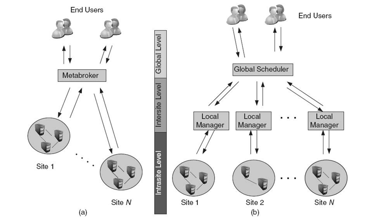
FIGURE 20.1. Two-level (a) and three-level (b) hierarchical architectures of the cluster in a computational grid.

Different types of scheduling problems in grids are generated by the various configurations of the main scheduling attributes, where the system architecture, task processing policy, and interrelations among tasks in the users'applications are the major characteristics [7, 9]. This chapter addresses an independent grid job scheduling, where tasks are executed independently of each other and are processed in the batch mode. This means that the whole batch is scheduled as a group of tasks. The problem is formalized by using an expected time to compute (ETC) matrix model [15]. Let us denote by n a number of tasks in the batch and by m a number of machines available in the system. An instance of the problem in this model is defined by the following set of the input data:

• a workload vector for tasks in the batch, W = [w₁,…, w_n], where w_j denotes the computational load of the task j expressed as a number of computational cycles needed for completion of this task
• a vector of speed parameters for the machines, S = [s₁,…, s_m], in which s_i denotes the frequency of machine i defined as the number of computational cycles per time unit (second)
• a ready times vector, ready times = [ready₁,…, ready_m], where ready_i is the time needed for reloading the machine m_i after finishing the last assigned task to make this machine ready for the further assignments
• an expected time to compute (ETC) matrix, ETC = [ETC[j][i]]_n×m, of expected (estimated) times of the tasks on machines calculated for all possible task‒machine pairs.

In the simplest case, the elements of the ETC matrix can be computed by dividing the workload by computational load for each task‒machine pair, that is, ETC[j][i] = w_j/s_i.

Tasks in this model may be considered as monolithic applications or metatasks with no dependencies among the components. The workloads of tasks can be estimated based on specifications provided by the users or on historical data, or can be obtained from system predictions [16]. The term “machine” refers to a single or multiprocessor computing unit or even to a local small-area network.

20.3   GENERAL CHARACTERISTICS OF THE OPTIMIZATION LANDSCAPE

The theory of global optimization landscapes is needed for better understanding of the problems and the improvement of the performance of the search algorithms [2]. A fitness landscape can be formally defined as the following triplet:

where X represents the search space, N denotes a neighborhood operator, and f is a fitness function. It can be represented by a labeled graph, in which the vertices correspond to genotype solutions and edges connecting a pair of vertices indicate that each vertex is reachable from another with one application of the operator N. In the simplest case, the neighborhood of a given solution is generated based on an adjacency matrix defined for the landscape graph.

In grid scheduling, the search space is determined by the permutations of tasks or machine labels, but the lengths of these permutation strings may vary because the numbers of tasks and/or machines in the system can change over time. Therefore, additional probability distributions should be specified for an estimation of actual states of the system. The following two sections define basic components of two variants of the scheduling landscapes for CG, namely, large-scale static and dynamic grid landscapes.

20.3.1   Schedule Representation

The search space in the grid scheduling optimization landscape is determined by the set of all possible schedules generated for a given batch of tasks and the set of machines available in the system. Let us denote by N_l = {1,…, n} and M_l = {1,…, m} the sets of task and machine labels, respectively. Let Schedules denote the set of all permutations with repetitions of the length n over the set of machine labels M_l.

A schedule S ∈ Schedules is encoded by the following vector:

where i_j ∈ M_l is the number of machines to which the task labeled by j is assigned.

This encoding method is called a direct representation of the schedule S.

The lengths of the scheduling vectors are constant in the case of the static scheduling and can vary in the dynamic scenario. In the dynamic case, some additional probability distributions for modeling the changes of the system states (the changes in the numbers of tasks and machines) are needed. Therefore, the task labels in the dynamic scheduling are represented by the following set of parameters:

where init_t is the initial number of tasks in the system, max_t is the maximal number of tasks in the system, and E(inter_t) is the exponential probability distribution of the new tasks arrived to the system.

The machine labels in the dynamic scheduling are represented by the following parameters:

where init_m stands for the initial number of machines, min_m denotes the minimal number of machines, max _m denotes the maximal number of machines, G(add_m) is the Gaussian probability distribution [17] of adding (arriving) the machines to the system, and G(del_m) is the Gaussian probability distribution of removing machines from the system.

20.3.2   Scheduling Criteria

The grid scheduling problem is usually considered as the multiobjective optimization problem with numerous scheduling criteria and the scheduling objective functions [18]. The are two basic models used in grid multiobjective optimization: hierarchical and simultaneous modes. In the simultaneous mode, all scheduling criteria are optimized simultaneously. In the hierarchical case, different scheduling criteria are sorted a priori according to their importance in the model. The process starts by optimizing the most important objective function. When further improvements are not possible, the second objective function is optimized and the values of the first objective function are kept at the optimal level. The method proceeds until all criteria are optimized. It is very hard in grid scheduling to define or efficiently approximate the Pareto front, especially in dynamic scheduling.¹ This set of Pareto optimal solutions may extend very fast together with the scale of the grid and the number of the submitted tasks. The specification of the structure of the Pareto front is also an open problem in grid scheduling. Due to the sheer size of the grid itself and the huge number of possible schedulers even for a small amount of tasks, an effective and fast exploration of the search space for the problem is very difficult.

In this chapter, grid scheduling is defined as a bi-objective optimization problem with makespan and flowtime as the main criteria.

20.3.2.1   Calculation of the Makespan  Makespan is expressed as a finishing time of the latest task. It can be formally defined as follows:

where F_j denotes the time when task j is finalized.

Using the ETC matrix model, the makespan can be defined in terms of the completion times of the machines as the maximal completion time of the machines available for the batch of tasks. Let us denote by completion a vector of size m. The ith coordinate in this vector is denoted by completion[i] and indicates the total time needed for reloading the machine i after finalizing the previously assigned tasks and for completing the tasks actually scheduled to the machine. The completion[i] parameters can be calculated in the following way:

where T(i) is the set of tasks assigned to the machine i.

The makespan can be now expressed as follows:

20.3.2.2   Calculation of the Flowtime   The flowtime is expressed as the sum of finalization times of all the tasks. It can be defined in the following way:

Flowtime is usually considered as a quality of service (QoS) criterion. In terms of the ETC matrix model, the flowtime objective function can be calculated as a work-flow of the sequence of tasks on a given machine i, that is to say,

where sorted[i] denotes the set of tasks assigned to the machine i sorted in ascending order by the corresponding ETC values.

The cumulative flowtime in the whole system is defined as the sum of F[i] parameters; that is,

Both makespan and flowtime are expressed in arbitrary time units. In fact, their values are in incomparable ranges: Flowtime has a higher magnitude order over makespan, and its values increase as more tasks and machines are considered. Therefore, in this approach, the mean_flowtime = flowtime/m function is implemented for the evaluation of the flowtime criterion.

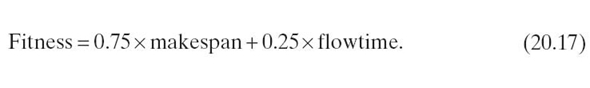
20.3.2.3   Cumulative Objective Function   The bi-objective scheduling problem is transformed into the mono-objective problem by aggregating the makespan and mean_flowtime functions into the following cumulative weight function:

The weight coordinate λ ∈ (0, 1) is used, in fact, for the specification of the priorities of the considered scheduling criteria. It is assumed that λ ≠ 0 and λ ≠1. Based on the experimental tuning results presented in Reference 19, the following three values of the λ coefficient are considered in the empirical analysis presented in Section 20.5: (1) λ = 0.25, (2) λ = 0.50, and (3) λ = 0.75.

20.4   MULTILEVEL METAHEURISTIC SCHEDULERS

The general characteristics of a grid scheduling fitness landscape usually depend on the features of the resolution method defined for the considered scheduling model. This section presents the characteristics of a generic model of a single-population genetic scheduler, which can be used independently as the scheduling algorithm or can be integrated with the general frameworks of hierarchical or hybrid genetic strategies. The general concepts of two multilevel grid schedulers, namely, HGS-Sched and a combination of genetic algorithm and tabu search (GA + TS) metaheuristics, are presented in Sections 20.4.2 and 20.4.3.

20.4.1   Single-Population Genetic Schedulers

The general model of a single-population genetic scheduler is based on the framework of the GAs used in the combinatorial optimization [20]. This model is also used as a basic genetic engine in numerous multipopulation and multilevel genetic schedulers. The general framework of this engine is defined in Figure 20.2. This method was adapted to the grid scheduling problem through an implementation of specialized encoding methods and genetic operators.

Beyond the direct representation of the schedules, defined in Section 20.3.1, another encoding method, namely, the permutation-based encoding method, is needed for the implementation of the specialized genetic operators. In this method, each schedule is represented by the following pair of vectors:

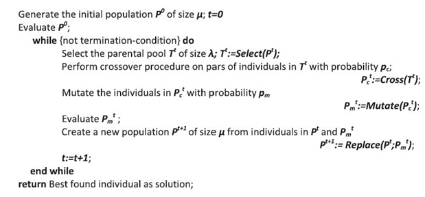
FIGURE 20.2. The general framework of the single-population genetic grid schedulers.

where u_i ∈ N_l, v_j = 1,…, n.

Vector u defines a permutation of task labels. It can be interpreted as a concatenation of the sequences of tasks assigned to particular machines. The tasks in these sequences are increasingly sorted with respect to their completion times. Information about the number of tasks mapped to each machine is encoded by vector v.

An initial population in GA defined in Figure 20.2 is generated by using the MCT + LJFR-SJFR method, in which all but two individuals are generated randomly. Those two individuals are created by using the longest job to fastest resource‒shortest job to fastest resource (LJFR - SJFR) and minimum completion time (MCT) heuristics [21]. In the LJFR-SJFR method, initially the number of m tasks with the highest workload is assigned to the available m machines sorted under the computing capacity criterion. Then, the remaining unassigned tasks are allocated in the fastest available machines. In the MCT heuristics, a given task is assigned to the machine yielding the earliest completion time.

The following genetic operators have been implemented in the main loop of the GA presented in Figure 20.2:

• Selection Operators. Linear ranking
• Crossover Operators. Partially mapped crossover (PMX), cycle crossover (CX)
• Mutation Operators. Move, swap
• Replacement Operators.Steady state, elitist generational.

All the above-mentioned operators are commonly used in the genetic metaheuristics dedicated to solving combinatorial optimization problems [22].

In the linear ranking method, a selection probability for each individual in a population is proportional to the rank of the individual. The rank of the worst individual is defined as zero, while the best rank is defined as pop_size − 1, where pop_size is the size of the population.

In partially mapped crossover (PMX), a segment of one parent chromosome is mapped to a segment of the other parent chromosome (corresponding positions) and the remaining genes are exchanged according to the mapping relationship. The main idea of the CX is that each task in a chromosome must occupy the same position so that only interchanges between alleles (positions) can be made. First, a cycle of alleles is identified. The crossover operator leaves the cycles unchanged, while the remaining segments of the parental strings are exchanged.

In the move mutation, a task is moved from one machine to another one. Although the task can be appropriately chosen, this mutation strategy tends to unbalance the number of jobs per machine. In the swap mutation, the number of tasks assigned to the given machine remains unchanged, but two tasks are swapped in two different machines.

The base population for a new GA loop may be defined by using the elitist generational replacement method, where a new population contains two best solutions from the old base population and the rest are the newly generated offsprings. A steady-state strategy is implemented as an alternate replacement technique. In this method, the set of the best offsprings replaces the worst solutions in the old base population.

20.4.2   Hybridization of the GA Scheduler with TS

One important feature of genetic-based metaheuristics is that they can be easily hybridized with another optimization method. There are two main aspects that should be taken into account in designing the effective hybrid models: (1) a selection criterion for hybrid components and (2) a hybridization level. The first issue refers to two different types of the optimization techniques that are hybridized, namely,

• metaheuristic + metaheuristic, where both combined methodologies are meta-heuristics, and
• metaheuristic + local search method, where a metaheuristic is hybridized with a low-cost, deterministic, or stochastic local search algorithm.

The hybridization level issue refers to the methods of the implementation of the hybrid structure and the cooperation of the hybridized modules. The components in the combined algorithms may be strongly coupled, which means that the hybridized metaheuristics interchange their inner procedures. In the case of loosely coupled combination, the flow of each algorithm remains unchanged and both methods are executed one after another. One component in the hybrid structure can be selected as a control strategy and can play the role of the main unit in the system. The second method in such a system supports the main algorithm. Finally, all hybrid components can be executed sequentially or simultaneously.

In this work, the classical GA-based scheduler presented in the previous section has been combined with the TS method. TS is a metastrategy for guiding known heuristics to overcome local optimality (premature convergence) in global optimization [23]. It can be viewed as an iterative technique that explores the set of problem solutions by periodical “modification” of the set of solutions by using the neighbor solutions (located in the neighborhoods of the solutions from a given set) in order to improve the quality of the search procedure. The GA presented in Figure 20.2 is defined as the control metaheuristic, and the TS algorithm is implemented as a supporting metaheuristic to replace the mutation operation; that is, selection, crossover, and mutation in GA is replaced by selection, crossover, and TS procedures. Figure 20.3 depicts a general flow of the proposed GA + TS hybrid scheduler.

A generic pseudocode of the TS module is defined in Figure 20.3 [6].

The TS algorithm is activated for a population generated by the application of the crossover procedure in GA. The structure of this population is modified by the TS algorithm by replacing the current schedules by their better neighbor solutions if this replacement improves the fitness values of the solutions.

The important component of the TS method is a historical memory module, which consists of a short-term memory list with information on recently visited solutions and a long-term memory list for collecting the information gathered during the whole exploration process. The “movements” in these two lists cannot be activated, which means that their status is “tabu.” Therefore, some aspiration criteria are needed for eliminating the tabu movements from the memory component. Additionally, some local search inner heuristics are needed for an exploration of a neighborhood of a given solution. The intensification and diversification procedures can be activated for the management of the exploration/exploitation trade-off in the global search.

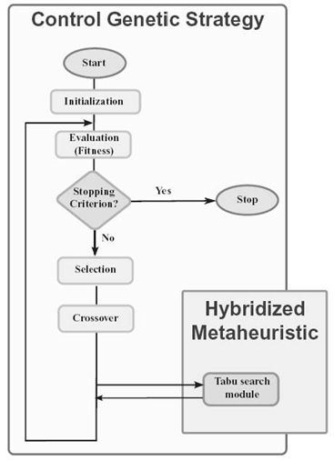
FIGURE 20.3. Model of a hierarchic GA + TS grid scheduler.

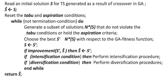
FIGURE 20.4. A template of tabu search module in hybrid genetic grid schedulers.

In this chapter, the following configuration of the TS algorithm is specified:

• Historical Memory. Both short- and long-term memories are used. For the recency memory, a tabu list matrix TL_(n×m) is generated to maintain the tabu status. In addition, a tabu hash table (TH) is used in order to further filter the tabu solutions.
• Neighborhood Exploration. Steepest descent/mildest ascent method with swap moving strategy, which exchanges two tasks assigned to different machines [24].
• Aspiration Criterium. GA fitness function.
• Intensification. This procedure is executed for the detailed exploration of promising regions in the optimization landscape by rewarding (attributes of) the current solution. The structure of the neighborhood of a given solution is modified by performing all possible swap movements between two machines and just one transfer from one machine to the other [23].
• Diversification. A soft diversification method is realized by using a penalization of ETC values technique, and a strong diversification method is realized by random modifications in the assignments of a sufficient number of tasks.

20.4.3   Hierarchic Genetic Strategy Scheduler (HGS-Sched)

HGS-Sched [11] is a multilevel genetic-based global optimization technique that enables a concurrent search in the grid environment by the simultaneous execution of many dependent evolutionary processes. This dependency relation is modeled as the multilevel decision tree with a restricted number of levels. Figure 20.5 depicts a simple graphical representation of three levels of HGS-Sched.

Each active evolutionary process is interpreted as a branch in this structure. The root of the tree is created by the algorithm of the lowest accuracy, which governs the search process and is responsible for the detection of promising regions in the optimization domain. Thereafter, more accurate processes are activated in those regions. The accuracy of search in HGS-Sched branches is defined by a degree parameter with the lowest value, for example, 0, set for the root of the system.²

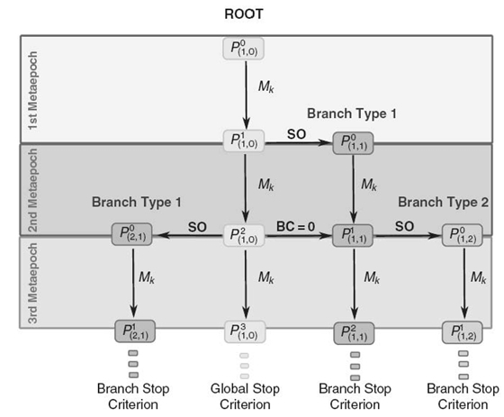
FIGURE 20.5. Three levels of the HGS-Sched tree structure.

The hierarchical structure of the scheduler is updated periodically after the execution of k-generation evolutionary processes in each active branch. Such a process is called a k-periodic metaepoch M_k, (k ∈ ℕ) and is defined in the following way:

where is the best adapted individual in the metaepoh, denotes a population evolving in the branch of degree t, e is the global metaepoch counter, M is the maximal degree of a branch, and r is the number of branches of the same degree.

New branches of the higher degree are created by using a sprouting operation (SO) defined follows:

where is a parental branch and denotes an initial population for a new branch of degree (t + 1). Individuals to this population are selected from an s_t-neighborhood (1 ≤ s_t ≤ n) of the best adapted individual in the parental population . This neighborhood is created by all possible permutations or reassignments of tasks in (n − s_t)-length suffix of The values of s_t parameters may be different in branches of the different degrees. In this work, the lengths of suffixes are calculated in the following way:

where suf ∈ [0, 1] is a global strategy parameter called a neighborhood parameter and t is the branch degree.

The sprouting operation is conditionally activated depending on the outcome of a branch comparison (BC) binary operator applied for parental and its all directly sprouted branches. It is used for the detection of “similarity” of the resulting populations in each parental-sprouted pair of branches. The outcome of the BC operator is 1 if the parental branch and its “descendant” (sprouted) branch operate in a similar region in the optimization landscape. In such a case, another metaepoch is executed in the parental branch without creating any new process. This technique is crucial in an effective management of the algorithm structure by preventing the activation of many similar processes in the same local region, which usually increase significantly the complexity of the whole strategy.

Similarity of populations can be estimated by using the hash technique to reduce the execution time of the BC procedure. The main procedure in the hash method is a hash table with the task‒resource allocation key denoted by K. The value of this key is calculated as the sum of the absolute values of the subtraction of each position and its precedent in the s_t-length suffix in direct representation of the schedule vector (reading the suffix in a circular way). The hash function f_hash is defined as follows:

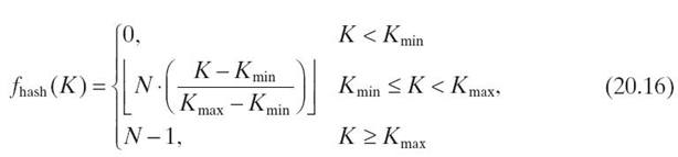
where K_min and K_max, respectively, correspond to the smallest and the largest value of K in the population and N is the population size.

In the case of the conditional sprouting of the new branches of the degree (t + 1) from the parental branch of the degree t, the keys are calculated for the best individual in the parental branch and individuals in all populations in all active branches of the degree (t + 1). If there is any individual in the higher-degree branches, for which the key matches the key of the best adapted individual in the parental branch, then the value of BC is 1 and no branch of the degree (t + 1) is sprouted.

In the case of the comparison of the branches of the same degree t, all branches, in which there exists the individuals with the identical keys, have to be reduced and a single joint branch is created (the value of BC is 1). The individuals in this branch are selected from the “youngest” (in the sense of the population evolution) populations in all reduced branches.

20.5   EMPIRICAL ANALYSIS

All considered metaheuristics have been integrated with a discrete event-based HyperSim-G [25] grid simulator for the purpose of the empirical comparative evaluation of the performance of single- and multilevel genetic schedulers. Based on the idea of the ETC matrix model presented in Section 20.2, the simulator creates an instance of the scheduling problem by using the following input data: (1) workload vector of tasks, (2) computing capacity of machines, (3) prior load of machines, and (4) the ETC matrix. The defined instance is passed on to the scheduler's module, which computes or estimates the optimal solutions of the scheduling problem. Finally, the scheduler sends back the information about planned assignment of tasks to the simulator, which provides the resource allocation.

The instances generated by the simulator are divided into static and dynamic grid scheduling benchmarks. In the static case, the number of tasks and the number of machines remain constant during the simulation, while in the dynamic case, both parameters may vary over time. In both static and dynamic cases, four grid size scenarios are considered: (1) “small” (32 hosts/512 tasks), (2) “medium” (64 hosts/1024 tasks), (3) “large” (128 hosts/2048 tasks), and (4) “very large” (256 hosts/4096 tasks).

The simulator is highly parameterized in order to reflect the realistic grid scenarios. The main parameters are defined as follows:

• Number of Hosts. Number of resources in the environment
• Cycles. Normal distribution modeling computing capacity of resources
• Total Tasks. Number of tasks to be scheduled
• Workload. Normal distribution modeling the workload of tasks
• Host Selection. Selection policy of resources (all means that all resources of the system are selected for scheduling purposes)
• Task Selection. Selection policy of tasks (all means that all tasks in the system must be scheduled)
• Number of Runs. Number of simulations done with the same parameters. Reported results are then averaged over this number.

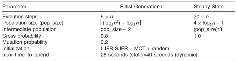
Table 20.1. Values of Key Parameters of the Grid Simulator in Static and Dynamic Cases

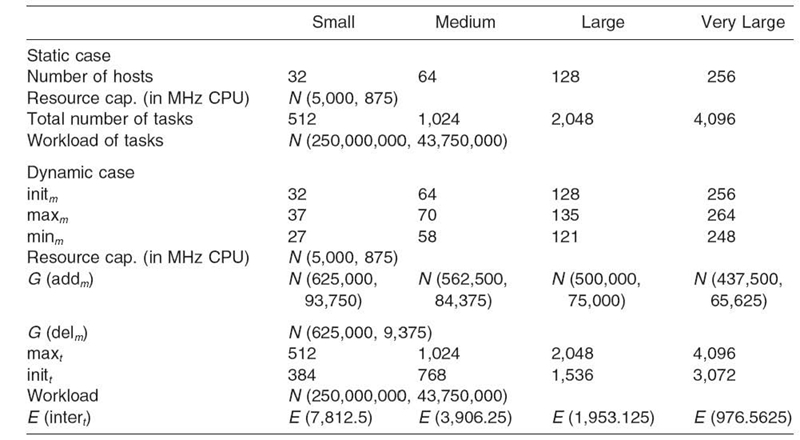
Table20.1 presents the key input parameters of the simulator in static and dynamic cases.³

All experiments in this section are scheduled as follows. In the first part of the analysis are eight possible variants of the standard GA-based schedulers defined in Section 20.4.1 with different crossover, mutation, and replacement operators in order to compose an optimal combination of genetic operations. This tuning of the main operators in GA is necessary for the design of the efficient genetic engine in both proposed multilevel schedulers—HGS-Sched and GA + TS hybrid algorithms. The experimental comparative evaluation of these methods and simple statistical analysis of the results are performed as the main part of the multilevel exploration of the grid scheduling landscape.

20.5.1   Tuning of the GA Engine

The analysis starts with tuning the genetic operations in single-population GAs and the weight coordinates in the fitness function defined in Equation (20.11). The configurations of the genetic operators for eight variants of single-population GAs are presented in Table 20.2.

Table 20.2. Eight Variants of GA-Based Grid Schedulers

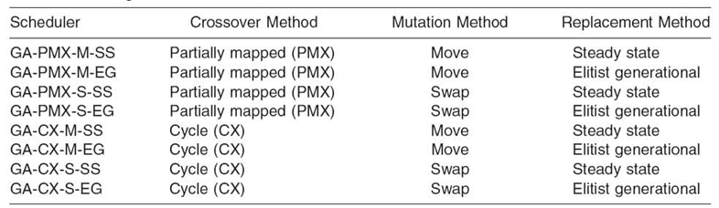
Table 20.3. GA Setting for Large Static and Dynamic Benchmarks

The values of key parameters for each scheduler are presented in Table 20.3.

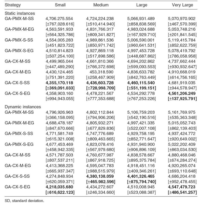
Eight GA metaheuristics were evaluated in static and dynamic grid environments. Each experiment was repeated 30 times under the same configuration of operators and parameters. Tables 20.4‒20.6 present the average fitness values achieved by all schedulers for the following weight parameters (see Equation 20.11): λ = 0.25, λ = 0.50, and λ = 0.75. All results are expressed in arbitrary time units (not necessary milliseconds or seconds).

The best results in the fitness minimization achieved by all considered meta-heuristics are observed in the case of λ = 0.75. It means that makespan is defined as the dominant scheduling criteria. The fitness function is defined as follows (see Equation 20.11):

The weight coordinate in the fitness function is three times higher for makespan than for flowtime.

It follows from the results presented in Table 20.6 that the algorithms with the steady-state replacement mechanism are three times more effective in the makespan minimization than the other schedulers. Particularly in the dynamic case, the combination of steady-state replacement with CX crossover and swap mutation seems to be an optimal configuration for a genetic makespan optimizer.

In the case of the flowtime optimization, the GA-CX-S -SS algorithm outperforms the other techniques in dynamic scheduling, which is the most realistic scenario in grid computing.

Table 20.4. Average Fitness Values for λ = 0.25, [ ± SD]

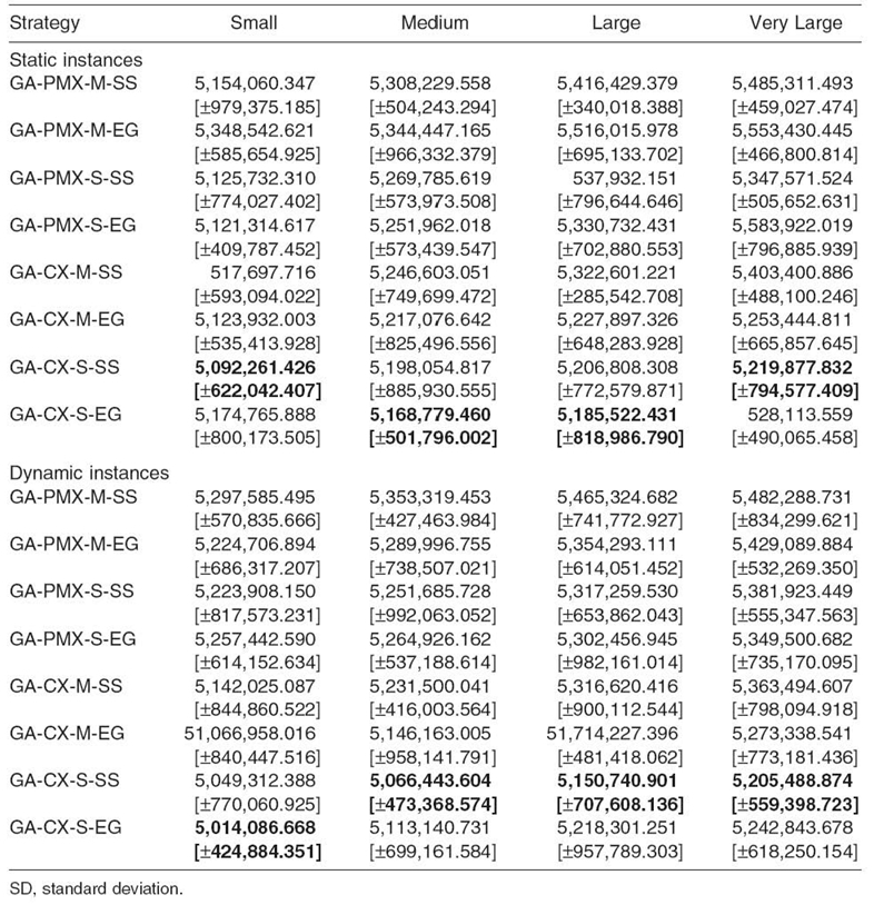
Based on the fitness results, the GA-CX-S-SS algorithm is selected as the most effective single-population scheduler, and it is implemented as the genetic engine for the empirical analysis of multilevel grid scheduling presented in the following section.

20.5.2   Empirical Evaluation of Single-Population Scheduler, HGS-Sched, and GA + TS Hybrid Metaheuristic in Static and Dynamic Grid Environments

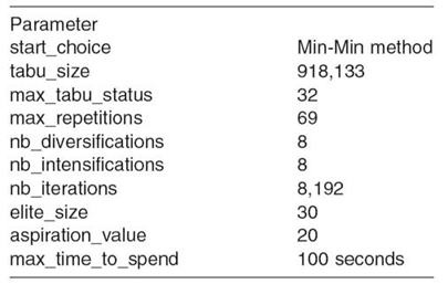
The objective of the study presented in this section is to verify and compare the efficiency of the best single-population genetic scheduler generated in the previous section, namely, GA-CX-S-SS, HGS-Sched, and GA + TS algorithms in the exploration of the complex grid scheduling landscape. The GA-CX-S-SS algorithm has also been implemented as the basic genetic mechanism in the multilevel metaheuristics. Table 20.7 and Table 20.8 present the key parameters of HGS-Sched and GA + TS.

Table 20.5. Average Fitness Values for λ = 0.50 [ ± SD]

It is assumed that HGS-Sched tree is composed of the branches of degrees 0 and 1, and the search process in the sprouted branches is approximately two times slower than in the core (the mutation rate in the sprouted branches is just a half of the mutation rate in the core). Also, the populations in the sprouted branches are much smaller than a global population in the core of the tree, which is crucial in the efficient local exploration of the genetic optimization landscape. In the case of elitist-like replacement mechanisms, small populations can escape much faster from the basin of attractions of a local solution compared with the big sets of individuals.

In the TS algorithm, the size of the tabu hash table (TH) is set to 918,133, as it is recommended by Srivastava [26]. The maximum number of iterations a solution remains tabu (max_tabu_status) is generated uniformly from the interval [m, 2 · m] (m—number of machines), and the maximum number of successive iterations without improvements of the current solution implying the activation of the intensification is fixed to 4 ln(n) · ln(n). The number of iterations of the diversification and the intensification procedures are set to log₂(n). Finally, 30 elite solutions are kept in each iteration, and the parameter (max_tabu_status/2) − log₂(max_tabu_status) defines the minimum number of iterations after which the tabu movement can aspire. The algorithm runs for 100 seconds (a realistic runtime for scheduling tasks in grids).

Table 20.6. Average Fitness Values for λ = 0.75 [ ± SD]

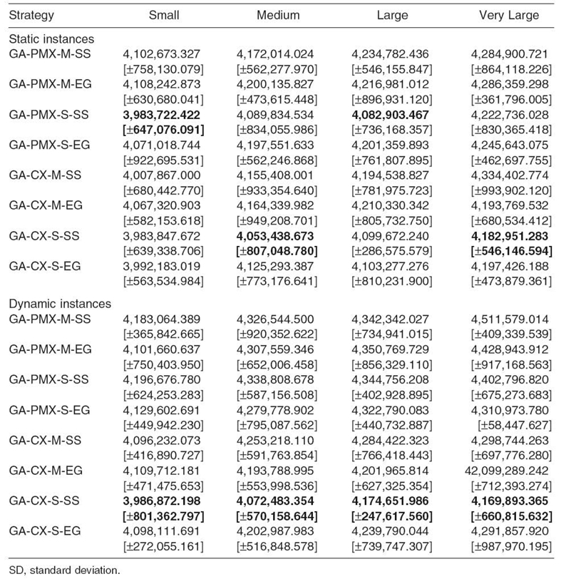
Table 20.7. HGS-Sched Settings for Static and Dynamic Benchmarks

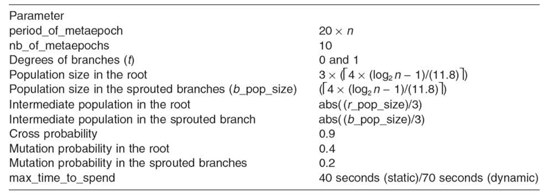
Table 20.8. Parameterization of TS Algorithm

Each experiment has been repeated 30 times under the same configuration of operators and parameters. The weight coordinate in the fitness function is λ = 0.75. The average makespan and flowtime values achieved by three genetic schedulers are presented in Figure 20.6.

It can be observed that the effectiveness of both schedulers in flowtime optimization is in the same range; the differences in the results are very minor. The analysis of the makespan reduction is much more interesting. The GA + TS hybrid scheduler is more efficient in the static case. It may stem from the fact that TS technique may be an appropriate methodology for an accurate exploration of the highly parametrized local static neighborhoods of the temporary solutions found by the genetic steering module. However, this technique may be sensitive on any modifications of the system state. The TS metaheuristic cannot guarantee a fast escape from a basin of attraction of already detected local optima in the case of appearance of new promising solutions. Therefore, in the dynamic scenario, the HGS-Sched algorithm seems to be better adapted for an exploration of new regions in the optimization landscape. Finally, we observed that both multilevel schedulers outperform the single-population GA-CX-S-SS scheduler in all considered instances.

20.5.2.1   Statistical Analysis of the Results   The results presented in Figure 20.6 give us just a general information about the schedulers'performances. In order to make our comparison analysis more reliable, we calculated a coefficient of variation and performed Student's t-test for means for the verification of the statistical significance of the results.

20.5.2.2   Coefficient of Variation   The coefficient of variation (CV) [17] is defined as the statistical measure of the dispersion of data around the average value. It expresses the variation of the data as a percentage of its mean value and is calculated as follows:

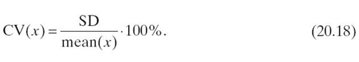
CVs calculated for stable heuristic methods should not be greater than 5%. Table 20.9 presents the coefficients of variation calculated for all makespan and flowtime results achieved by GA-CX-S-SS, HGS-Sched, and GA + TS schedulers.

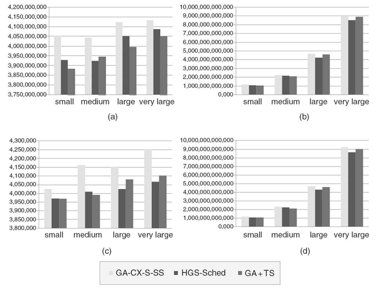
FIGURE 20.6. Experimental results achieved by GA-CX-S-SS, HGS-Sched and GA + TS schedulers: in static case—(a) average makespan, (b) average flowtime; in dynamic case—(c) average makespan, (d) average flowtime.

It can be observed that, in all instances, the values of CVs for HGS-Sched and GA + TS algorithms are in the range 0−3.2%, which confirms the stability of those metaheuristics. The values of CVs calculated for GA-CX-S-SS algorithms are in [5.87; 13.08], which shows the low stability of this scheduler.

20.5.2.3   Student's t-Test for Means   A simple comparison of the averaged values of the scheduling objective functions and the standard deviations is usually insufficient to measure the relative performance of the schedulers. Therefore, the standard Student's t-test for the comparison of two means [17] was used for the verification of statistical significance of all empirical results of minimization of makespan and flowtime. The result of this test is the acceptance or rejection of the null hypothesis (H0), which states that any differences in results are purely random. An erroneous rejection of the null hypothesis defines a type 1 error.

Table 20.9. Comparison of the Coefficients of Variation (CV for Makespan and Flowtime Values in the Large Size Static and Dynamic Instances (All Values in %)

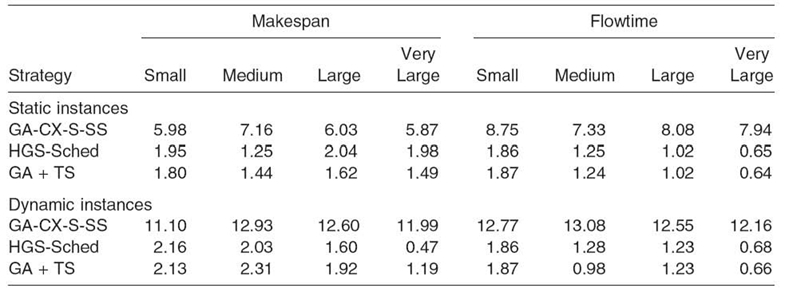
Table 20.10. Comparison of the Two-Tailed p-Values for Makespan and Flowtime Results in the Large Size Static and Dynamic Instances

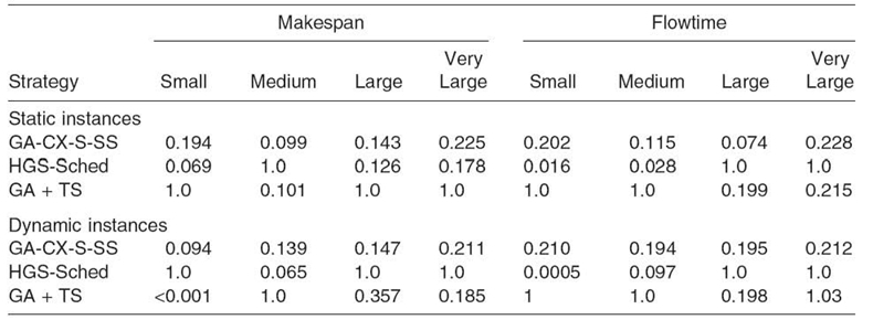
The best achieved makespan and flowtime values in each problem instance have been defined as the reference values in the verification of the “null” hypothesis, and the confidence level was 95% in each instance of the t-test.

Table 20.10 shows the probabilities of type 1 errors (p-values) [17]. The difference in results is not statistically significant if the p-value is not greater than 0.05 (p-value is 1 for the base (best) results to which the remaining results are referred).

In the static instances, HGS-Sched is better than GA + TS hybrid in the case of medium grid size for makespan, and large and very large grids for flowtime. The differences in results achieved by two multilevel metaheuristics in all instances but large and very large grids for flowtime are statistically significant, which means that in the static scenario, HGS-Sched is more effective in flowtime reduction, while GA + TS outperforms the hierarchical algorithm in the makespan minimization. The situation is different in the dynamic scenario, where the higher effectiveness of HGS-Sched is demonstrated in all but the medium grid case. In all cases, the results achieved by the single-population algorithm are significantly worse than the results generated by the two multilevel schedulers.

20.6   CONCLUSIONS

This chapter presents the empirical analysis of three different techniques of exploration of the bi-objective fitness landscape for independent grid scheduling. The first methodology is based on the hybrid two-level search of GA and TS algorithms. GA plays a role in the control strategy, while TS in the subordinated module is responsible for the accurate exploration of the neighborhoods of suboptimal schedulers detected by GA. The results of experiments show the high effectiveness of this metaheuristic in static scheduling. Indeed, the TS component is successful in the fast reduction of the main objective (makespan). It can also distinguish the similar (optimal) solutions distributed in the small narrow regions of the search space. On the other hand, the major drawback of this method may be the low resistance to the system dynamics. In such cases, the hierarchical genetic strategy outperforms the other similar approaches. Both multilevel metaheuristics achieved better results that single-population schedulers. It seems that local search in some promising regions in the optimization landscape or concurrent exploration of this landscape by many dependent genetic processes with various accuracy of search is more effective in the large-scale dynamic combinatorial optimization than conventional genetic methodologies.

Similar to the classical combinatorial optimization, even a simple theoretical analysis of the scheduling landscapes in CGs may be a strong support to the design of the scalable grid schedulers that can be easily adapted to actual system states. This research area is still very superficially explored, and each progress in the landscape characteristics may be the hottest research issue in future generation grid and cloud computing.

REFERENCES

[1] E.-G. Talbi and A.Y. Zomaya, Grids for Bioinformatics and Computational Biology. Hoboken, NJ: John Wiley & Sons, 2007.

[2] P. Stadler, Towards a theory of landscapes in Complex Systems and Binary Networks (R. Lopéz-Peña et al., ed.), Lecture Notes in Physics, Berlin: Springer Verlag, pp. 77‒163, 1995.

[3] M. Maheswaran, S. Ali, H.J. Siegel, D. Hensgen, and R.F. Freund, “Dynamic mapping of a class of independent tasks onto heterogeneous computing systems,” Journal of Parallel and Distributed Computing, 59: 107‒131, 1999.

[4] C.R. Reeves, “Landscapes, operators and heuristic search,” Annals of Operations Research, 86: 473‒490, 1999.

[5] D. Whitley and S., Rana and R.B. Heckendorn “The island model genetic algorithm: On separability, population size and convergence,” Journal of Computing and Information Technology, 7: 33‒47, 1998.

[6] F. Xhafa, J. Carretero, E. Alba, and B. Dorronsoro, “Tabu search algorithm for scheduling independent jobs in computational grids,” Computer and Informatics, Special Issue on Intelligent Computational Methods, J. Burguillo-Rial, J. Kołodziej and L. Nolle, eds., 28(2): 237‒249, 2009.

[7] A. Abraham, R. Buyya, and B. Nath, “Nature's heuristics for scheduling jobs on computational grids,” in Proceedings of the 8th IEEE International Conference on Advanced Computing and Communications, India, pp. 45‒52, 2000.

[8] J. Kołodziej and F. Xhafa, “Meeting security and user behaviour requirements in grid scheduling,” Simulation Modelling Practice and Theory, 19(1): 213‒226, 2011.

[9] J. Kołodziej and F. Xhafa, “Enhancing the genetic-based scheduling in computational grids by a structured hierarchical population,” Future Generation Computer Systems, 27: 1035‒1046, 2011.

[10] J. Kołodziej, R. Gwizdała, and J. Wojtusiak, “Hierarchical genetic strategy as a method of improving search efficiency,” in Advances in Multi-Agent Systems (R. Schaefer and S. Sedziwy, eds.), Cracow: UJ Press, pp. 149‒161, 2001.

[11] R. Schaefer and J. Kołodziej, “Genetic search reinforced by the population hierarchy,” in FOGA VII, Morgan Kaufmann, pp. 383‒401, 2003.

[12] J. Kołodziej and M. Rybarski, An application of hierarchical genetic strategy in sequential scheduling of permutated independent jobs. in Evolutionary Computation and Global Optimization (J. Arabas ed.), Vol. 1. Warsaw: Warsaw University of Technology, Lectures on Eletronics, pp. 95‒103, 2009.

[13] J. Kołodziej, W. Jakubiec, M. Starczak, and R. Schaefer, “Hierarchical genetic strategy applied to the problem of the coordinate measuring machine geometrical error,” in Proceedings of the IUTAM '02 Symposium on Evolutionary Methods in Mechanics, pp. 22‒30, Cracow, Poland, Kluver Ac. Press, September 24‒27, 2002, 2004.

[14] R. Buyya and K. Bubendorfer eds., Market Oriented Grid and Utility Computing. Hoboken, NJ: Wiley, 2009.

[15] S. Ali, H.J. Siegel, M. Maheswaran, S. Ali, and D. Hensgen, “Task execution time modeling for heterogeneous computing systems,” in Proceedings of the Workshop on Heterogeneous Computing, pp. 185‒199, 2000.

[16] S. Hotovy, “Workload evolution on the cornell theory center IBM SP2,” in Proceedings of the Workshop on Job Scheduling Strategies for Parallel, IPPS '96, pp. 27‒40, 1996.

[17] P.S. Mann, Introductory Statistics, 7th ed. Hoboken, NJ: Wiley, 2010.

[18] E.-G. Talbi, Metaheuristics: From Design to Implementation. Hoboken, NJ: John Wiley & Sons, 2009.

[19] F. Xhafa, E. Alba, B. Dorronsoro, and B. Duran, “Efficient batch job scheduling in grids using cellular memetic algorithms,” Journal of Mathematical Modelling and Algorithms, 7(2): 217‒236, 2008.

[20] Z. Michalewicz, Genetic Algorithms + Data Structures = Evoluation Programs. Berlin: Springer Verlag, 1992.

[21] F. Xhafa, J. Carretero, and A. Abraham, “Genetic algorithm based schedulers for grid computing systems,” International Journal of Innovative Computing, Information and Control, 3(5): 1053‒1071, 2007.

[22] L. Davis, ed., Handbook of Genetic Algoriithms. New York: Van Nostrand Reinhold, 1991.

[23] F. Glover and M. Laguna, Tabu Search. Norwell, MA: Kluwer Academic Publishers, 1997.

[24] A. Thesen, “Design and evaluation of tabu search algorithms for multiprocessor scheduling,” Journal of Heuristics, 4(2): 141‒160, 1998.

[25] F. Xhafa, J. Carretero, L. Barolli, and A. Durresi, “Requirements for an event-based simulation package for grid systems,” Journal of Interconnection Networks, 8(2): 163‒178, 2007.

[26] B. Srivastava, “An affective heuristic for minimising makespan on unrelated parallel machines,” Journal of the Operational Research Society, 49(8): 886‒894, 1998.

 

¹A solution is Pareto optimal if it is not possible to improve a given objective function without deteriorating at least another one [18].

²The HGS-Sched framework may be used for the implementation of the single-population genetic algorithms and evolutionary strategies. In such a case, the tree is created by just one branch (root).

³See Section 20.3.1. The notations N (a, b) and E (c, d) are used for Gaussian and exponential probability distributions.