23

–––––––––––––––––––––––

A Survey of Techniques for Improving Search Engine Scalability through Profiling, Prediction, and Prefetching of Query Results

C. Shaun Wagner, Sahra Sedigh, Ali R. Hurson, and Behrooz Shirazi

23.1   INTRODUCTION

Search engines are vital tools for handling large repositories of electronic data. As the availability of electronic data continues to grow, search engine scalability gains importance [1]. As noted in the literature, researchers have measured search engine performance in terms of response time and relevance [2‒5], both of which suffer as the number of potential search results increases. Response (or search) time is the time elapsed between initiation of a query and when the desired data item is available to the user. Relevance quantifies the relevance of the results returned. Search engines typically exhibit a trade-off between response time and relevance [6]. However, irrelevant search results (even when delivered quickly) require that the query be refined and repeated, increasing the overall search time [2]. This chapter presents a survey of techniques that can be used to increase the relevance and to reduce the response time of search engines by predicting user queries and prefetching the results.

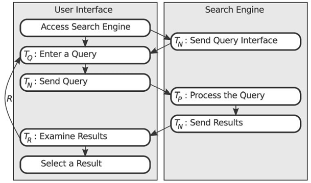
FIGURE 23.1. Operational fl ow of a standard query‒response search engine.

When a user is querying for a specific item, such as a book title, searching an information repository is a trivial task of carrying out an equality search on an index, that is, metadata. There is little room for improvement in response time or relevance. In practice, users often carry out searches with only a vague description of a topic or concept. In this case, the user attempts to form a descriptive query of what he or she is looking for, and it is up to the search engine to determine the semantics of the request and to generate query results that best match the semantic concept of the query. If this determination is made incorrectly, the search results returned will be irrelevant, necessitating that the user refine and repeat the query. This query‒response system, depicted in Figure 23.1, is the basis of all popular search engines [3, 4].

Equation (23.1) expresses the total search time (T_T) as a sum of the time spent on each independent step of the search process: query entry time (T_Q), query processing time (T_P), and search result examination time (T_R). If the search results are not acceptable, the entire process is repeated R times:

Network access time, for example, network latency (T_N), is repeated in Equation (23.1): to represent a need to access the search engine interface, to send the query to the search engine, and to send the results back to the user. Normally, when a server sends a result list to the user, it also displays the query interface. Therefore, the initial network access time is not repeated on successive queries. Very little data are communicated between the client and servers throughout the query processing time, limiting the benefit of reducing T_N to increase scalability. Furthermore, reduction of T_N is primarily related to hardware, not software. As such, we will omit network access time from the total search time for the remainder of this chapter.

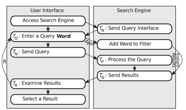
FIGURE 23.2. Google Instant displays search results after each word typed. The user may select a result at any time.

Traditionally, search engine improvement was primarily due to improved indexing techniques, which by default decreased the time spent processing the query and displaying relevant search results (T_P) [4]. Recent advances in search engine improvement are focused on query caching and methods designed to create an overlap between T_Q and T_P [7, 8]. The literature abounds with techniques and solutions for data caching in general, and web caching in particular, as a means to improve web searching. The speedup gain due to web caching is based on the fact that the results of popular search topics are often cached (see Appendix A.2). Caching the top searches and their results decreases the query processing time of similar future searches to a significant extent [3, 9].

Google visibly attempted to speed up the query process through Google Instant—a more interactive query entry process (depicted in Figure 23.2) [10]. Normally, search engine users are required to enter a complete query and to submit it to the server. This entry and submission time (T_Q) takes 9 seconds on average [4 , 10]. With Google Instant, Ajax is used to overlap the user]´s query entry time with the server´s query processing time. Each time the user presses the space bar, demarcating one word from the next, the query that has been entered so far is sent to the search engine for processing. Word by word, a result filter is produced and a running list of search results is displayed while the user continues to enter his or her query. By the time the user submits the complete query, most of the processing is complete. Google Instant is designed to avoid complete query entry. It is expected that the user will obtain a relevant result after only a portion of the query has been entered, eliminating the need for the remainder of the query entry process. In other words, network access (of duration T_N) + and query processing (of duration T_P) are performed during T_Q, for an average time reduction of 2‒5 seconds per search [10].

A further improvement in total search time would be to bypass the query entry and processing time (T_Q + T_N + T_P) and have immediate search results available to the user (see Figure 23.3). In this case, the user accesses the search engine. The search engine recognizes the user and while displaying a standard query interface, also displays a list of predicted search results. The user has the option to use the search interface to enter a query or can immediately select one of the predicted search results, saving about 10 seconds per query [10].

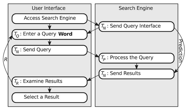
FIGURE 23.3. A predictive search engine sends predicted results along with the query interface.

While this predictive search engine would save time, a method of guiding users to information assumed relevant would redefine the way search engines are used [11]. Instead of having a complete idea and searching for information on the idea, a search engine can begin with the start of an idea and provide a list of results from other users´search histories, guiding the user through the search process that others have followed.

From the user´s point of view, prediction not only saves time but it also takes search engines beyond a simple search for information to a search for information from a sequence of related queries. The benefit of providing a sequence of search results can be shown in two scenarios. In the first example, a user sees an error message on a digital camera and wants to know what is wrong and how to fix it. In the second, an instructor is composing a sequence of topics for a course lesson plan.

In the first scenario, assume the user searches for a fix for an “E: 61: 10” error on a Sony DSC camera. Using both Google and Bing, the search results consist primarily of forum threads discussing the problem. It is possible that one of the threads will contain a solution to the problem, but searching through the threads is likely to be very time-consuming. Taking advice from forums may even result in damage to the camera because the solutions suggested include hitting the camera, smacking the camera on a desk, and soaking the camera in a bath of rubbing alcohol and bleach. However, E: 61: 10 is a common error for the Sony DSC camera, and as such, the search engine will have multiple records of other users searching for solutions to the very same error message. Instead of requiring the user to type the exact query needed to find a search result containing the solution, a predictive search engine will utilize these records to identify commonly selected destinations from other users ´ search histories—based on the assumption that useful solutions will be selected most often from among the search results returned. The user of the predictive search engine begins with a search for a solution to the camera´s error. The search results returned by the search engine will include a predicted path directly to the common destinations that contain a solution to the problem that led to initiation of the search.

In the second scenario, the instructor begins by searching for information about the initial topics for a course that he or she will teach. For example, the instructor first searches for information on vector algebra and selects a search result that appears promising. Then, the instructor searches for a dot product and selects another promising search result. The predictive search engine identifies the two previously selected search results and compares those to other user´s histories. Before the instructor begins another query, search results pertaining to cross product (the logical successor to the previous two topics) are shown. After selecting a destination from among the cross product results and returning to the search engine, search results pertaining to lines and planes are shown—before the instructor types a query. In this fashion, the search engine will present the instructor with a sequence of topics, that is, results from consecutive searches, that many others have utilized. This order is the logical order of topics for a majority of users. In this case, the instructor knows the destination for the course should be vector-valued functions, but is looking for the common sequence of topics, from beginning to end. In both scenarios, the power of the search engine is in prediction of user behavior based on the behavior of other users.

In the implementation of prediction, a search engine could either predict the query that the user will enter or predict the search result that the user will select. Prediction of search queries is less scalable than predicting selected search results. Many query terms are indexed for each search result, making the search space for queries exponentially larger than the search space for results [3, 11]. Consider the query “hedgehog information.” It yields search results for a small spiny mammal, a chocolate desert, and a spiked antisubmarine weapon—three very unrelated data items. Furthermore, if the search query is predicted, only the physical time spent typing the query will be saved. For example, the search engine will predict that the user will type “homes for sale in Albuquerque.” If the prediction is correct, the user submits the predicted query and gets the search results, just as if he or she had typed the query.

Unlike a query, a specific search result refers to a specific data item, for example, a URL for a web search engine or an image for an image search engine. By selecting a search result, the user is selecting a specific data item. Where prediction of a search query yields a vague prediction of multiple data items, prediction of a search result yields a specific data item. Therefore, the user ´ s selection from among search results is what should be predicted, as opposed to the search query itself.

Prediction is typically based on a model of user behavior, which is in turn based on profile information from multiple users. User behavior, within the realm of a search engine, is an ordered set of search results selected by him or her. With each user contributing a history of queries and (selected) search results, a vast collection of user histories is available for use in modeling and prediction of user behavior—in the context of this chapter, selection from among results returned in response to a query.

This chapter examines current methods of modeling and predicting user behavior. These methods use the behavior of multiple people to develop a model of user behavior. Then, the model (or models) is (are) used for prediction. Common methods are defined with examples as necessary. The rest of the chapter is organized as follows. Section 23.2 defines behavior modeling with examples. Often, a single model is incapable of accurately capturing the behavior of a population. In such cases, the population is divided into groups or neighborhoods, and the behavior of each is modeled separately. In Section 23.3, we discuss and analyze several grouping techniques, for example, k-nearest neighbor (KNN), a vector-based similarity method, and singular value decomposition (SVD). Algorithms for calculating a similarity value are used in both grouping and modeling. With rare exception, these algorithms fall under either vector- or string-based methods. Both techniques are examined in detail in Section 23.4. Vector methods generally require less processing time but lack accuracy. On the other hand, string-based methods are processing intensive but offer increased accuracy. Section 23.4.1 and 23.4.2 further analyze different vector- based and string-based methods, respectively. With user profiles grouped into neighborhoods of similarity, the next step in prediction is to develop a behavior model for each neighborhood. Given a target user, the neighborhood with users most similar to the target user is identified, and its behavior model is used in predicting the behavior of the target user. Section 23.5 is dedicated to this issue and serves to conclude the chapter and discuss future research directions.

23.2   MODELING USER BEHAVIOR

Both modeling and prediction of human behavior are established fields that gained popularity as psychology developed alongside early computers [12]. While the possibilities of human behavior appear to be infinite, the actual behavior of humans is limited by task goals and environment. Therefore, it is possible to describe human behavior as a sequence of dynamic states that can be captured by a state-space model. One such model is a Markov chain, which represents user behavior with a set of interconnected nodes [4]. Each node is a time-ordered action or observation. The weight of the directed link connecting two nodes represents the probability of transitioning from the first to the second, that is, that the action denoted by the destination node will immediately follow that of the source node. What differentiates Markov models from other state-space models is their memoryless feature: The next state only depends on the current state; that is, the current state subsumes the entire history of transitions.

Figure 23.4 is a model of user behavior at a vending machine. Many of the actions and observations are omitted, leaving only the most common actions and observations. User actions are in circles. User observations are in squares. Weighted arrows designate a transition from one state (be it an action or observation) to another by means of a user action. The weights (percentages) are the important part of the behavior model as they determine the likelihood of the transition. For example, 5 % of the time, a person would press the coin return directly after inserting change. After pressing a product button, the user will observe, 100 % of the time, either that an item is received or that nothing happens. The relative frequency of these two outcomes characterizes the behavior of the vending machine and, as such, does not appear in the user behavior model.

Given such a model, a computer can monitor user behavior and predict what the user´s upcoming actions and observations will be. If a user inserts change, there is a 95 % chance that the user will press a button to select an item. More complex predictions can be made, such as estimation of the probability that a user will press the coin return. After inserting change, there is a 5 % chance that a user will press the coin return. If the user presses a button to select an item, there is still a chance that the user will press the coin return, which is based on the chance that “nothing happens” will be observed by the user. Because “nothing happens” is an observation and not a decision for the user, the computer can monitor the vending machine to determine the probability of nothing happening. Assume that it is 10 %, and that the vending machine behavior is independent of that of the user—a reasonable assumption. Users who select an item will observe nothing happening 10 % of the time, and 85 % of those users will press the coin return. Therefore, 8.5 % of users who select an item will eventually press the coin return. The overall chance of the coin return being pressed is 13.5 %. Further, there is a possibility that those who press the coin return will observe that nothing happens. In this case, there is an 85 % chance that the user will press the coin return a second time.

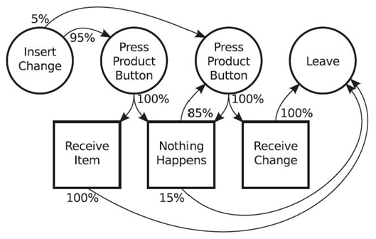
FIGURE 23.4. A model of typical user behavior at a vending machine.

This form of Markov modeling has been successfully tested for observation and prediction of complex human behavior. Toledo and Katz used a similar model to represent and accurately predict lane change behavior by automobile drivers [13]. While it is rare for drivers to change lanes in the exact same order or at the exact same location, the overall behavior was predicted by observing a specific driver ´ s actions and utilizing the Markov model that was developed by observing many other drivers.

Similarly, Pentland and Liu used Markov models to define general actions performed by automobile drivers [14]. They increased the accuracy of predictions by producing multiple Markov models. Drivers that exhibited similar behavior were clustered into similarity groups. A separate model was developed for each group. The models contained many common attributes but were different enough to clearly identify differences in behavior among the various similarity groups. New drivers were observed to produce a short history of their respective driving behaviors. That history was used to place each new driver in one of the similarity groups. Then, the model for that group was used to predict the driver´s behavior. The resulting predictions proved to be 95 % accurate.

23.3   GROUPING USERS INTO NEIGHBORHOODS OF SIMILARITY

When discussing prediction of user behavior, a common example is Amazon´s product recommendation algorithm. Customers recognize it as the “Customers Who Bought This Item Also Bought” feature. It is a popular and somewhat effective neighborhood model for collaborative filtering [15]. The goal is to identify objects by specific attributes and then use those attributes to cluster or group the objects by similarity. Each cluster is commonly referred to as a neighborhood. For Amazon, the customer´s attributes are the set of products purchased by the customer. Regardless of the similarity among the products purchased by a particular customer, customers whose respective search histories have considerable overlap are considered similar.

Metrics for search engine usage are abundant. As an example, Google has patented many of its measurements of search result relationships, such as keyword identification, hand ranking, geospatial relationships [16], and number of inbound links. Following Amazon´s model, search engine users who have selected a large number of the same search results are considered similar and should be grouped into a neighborhood of similarity in developing a predictive search engine.

23.3.1   Neighborhood Model

The KNN is commonly used to group objects into neighborhoods of similarity [17‒19]. Objects are characterized by a predefined set of simple attributes, often a small fraction of the attributes that could potentially characterize an object. The choice of attributes to include in this set greatly affects the usefulness of the resulting neighborhood model. Objects with similar attributes are grouped together. Once grouped, it is assumed that objects within the same neighborhood will share all attributes, including those not used in developing the neighborhood model.

As an example, the Piggly Wiggly grocery store may create neighborhoods of similarity based on the time of day a customer is most likely to make a purchase, the average cost of each purchase, and the specific store at which the purchase was made. From there, a neighborhood of morning shoppers who make purchases over $200 per trip to a beachside store may be identified as a neighborhood. With three simple attributes in common, Piggly Wiggly assumes that other attributes are shared. If a portion of customers in that neighborhood suddenly purchase a specific product, Piggly Wiggly can target marketing for the product to everyone in that specific group, instead of the general population. Obviously, Piggly Wiggly can use a more complex algorithm for grouping customers into neighborhoods, but the concept remains the same [20].

Regardless of application, the KNN algorithm can be broken into three simple steps. In these steps, a concept of distance is often used instead of similarity. Distance is a measure based on the attributes of two objects. The distance between two identical objects is zero. The larger the distance between two objects, the less similar the objects are. The term “distance” is derived from vector distance. Assuming that the attributes for an object are treated as a vector, the distance between the attribute vectors of two objects is the distance between the objects themselves. Common methods for determining distance are discussed in Section 23.4.

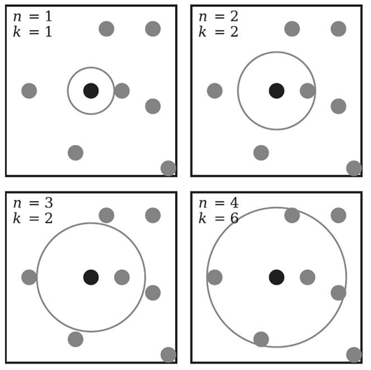
FIGURE 23.5. Effect of increasing the neighborhood radius (n) on the neighborhood cardinality (k).

To create a single neighborhood based on a target object within a large set of objects, the following steps are necessary:

1. Compute the distance from the target object to all other objects using predefined attributes.
2. Order the objects from least distant (similar) to most distant (different).
3. Select an optimal number (k) of nearest neighbors to include in the neighborhood of the target object. The value of k may be chosen beforehand or calculated based on an optimal neighborhood radius size [21]. See Figure 23.5 for examples of how the choice of neighborhood radius, n, affects the neighborhood size, k. Increasing n may or may not increase k.

An “object” may be any entity that will be modeled. For the purpose of collaborative filtering in a user‒product environment, some models cluster the users together, while others cluster the products. Amazon.com is an example of a successful collaborative filtering environment in which the users are compared to one another based on their respective purchasing histories, as in the “Customers Who Bought This Item Also Bought” feature [15]. Pandora.com is an example of a successful collaborative filtering environment in which the products, songs in this case, are matched by similarity across many metrics identified by the Music Genome Project [22]. Users who like one song are offered songs within the same neighborhood of similarity. Each approach (clustering users instead of products) has its own merits [23]. Users with similar attributes are likely to behave in a similar manner. Products with similar attributes are likely to be purchased (or perused) in a similar manner. It is also possible to have a complex grouping scheme that compares both users and products in determining neighborhoods of similarity.

23.3.2   SVD Model

It is often necessary to define a relationship between two sets of objects, such as customers and products. One method of doing so is to group each set of objects into neighborhoods of similarity, respectively, and then compare and contrast the various neighborhoods. The KNN algorithm is used to create a single neighborhood for a single object, not a set of neighborhoods for all objects. Further, the KNN algorithm is not capable of handling missing attributes—a common problem in real-world data.

Grouping and comparing objects is subject to several challenges—beyond missing attributes. These challenges include synonymy and polysemy. Synonymy occurs when two identical attributes have different names.Polysemy occurs when a single name refers to multiple attributes. To correct for missing data, synonymy, and polysemy, SVD has been widely used as a part of latent semantic indexing (LSI) [24] (see Section 23.4.1.2). Decreasing missing data, synonymy, and polysemy with SVD in turn increases the accuracy of grouping by similarity [25].

The purpose of SVD is to decompose a matrix M into three matrices that represent its rows, columns, and the relationship between the rows and columns, respectively. Specifically, SVD will convert an m × n matrix M into a collection of three matrices: an m × m unitary matrix U that describes the rows of M, an n × n unitary matrix V that describes the columns of M, and an m × n diagonal matrix Σ that describes the relationship between the rows and columns of M [26]. In practice, a thin form of SVD is implemented because it produces the same estimation with fewer calculations and values to store [27]. A thin SVD calculates only n columns of U and n rows of Σ. When compared to a full SVD, producing m columns of U and m rows of Σ does not provide a significantly more accurate result. The following example uses a thin SVD. With V^T denoting the conjugate transpose of V, the SVD of matrix M is defined as in Equation (23.2):

Relating this to users, assume each of three users, X, Y, and Z, is characterized by four attributes, a, b, c, and d. Matrix M, in Table 23.1, contains the attribute values for each user. Averaging the values of a single attribute over all three users produces the attribute average column U. The user average row V^T is produced by taking the average of the four attributes for each user.

TABLE 23.1. An Attribute Matrix Estimated by the Product of Two Matrices Containing Mean Average Values

TABLE 23.2. An Attribute Matrix Approximated by the Product of Two Matrices Containing Normalized Mean Values and a Scaling Factor

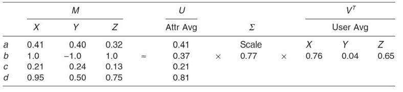
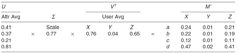
TABLE 23.3. Estimating the Original Matrix M

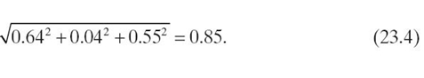
After calculating the average for all attributes and users (matrices U and V^T, respectively), the averages are normalized to place them on the same scale. The standard for doing so is to divide each value in a set by the square root of the sum of the square of each value in the set. Equations (23.3) and (23.4) show the calculation of the base for normalization of U and V^T, respectively.

Each value in U is divided by 0.91. Each value in V^T is divided by 0.85. The product of the two scaling factors, 0.77, forms the single-value matrix, Σ. As shown in Table 23.2, the original matrix, M, is estimated by the product of the three matrices, that is, U ΣV^T. Thus, the attribute and user matrices are normalized while the product of the two matrices, Uand V^T normalized, and the scaling factor, Σ, is the same as the product of the original U and V^Tmatrices.

At this point, it is important to note that the information originally represented as 12 separate values is now summarized in only eight separate values. By multiplying the average and scale matrices, an estimate of the original matrix can be produced as shown in Table 23.3.

The estimated matrix, M^', is radically different from the original matrix, M. This discrepancy arises from the inaccuracy resulting from the use of the mean as the averaging function. The sets of user or attribute values are vectors. The similarity between vector objects is dependent on vector angles, not magnitudes. Taking the mean values of the vectors of a matrix will usually change the angle of the norm of the matrix. Taking the eigenvalues of the vectors of a matrix will change the magnitude but not the angle of the norm of the vector. Therefore, using the eigenvalueas the averaging function maintains the similarity between the objects being compared. Repeating the above operations with eigenvalues produces the entries in Table 23.4.

TABLE 23.4. Producing U and V^T with Eigenvalues

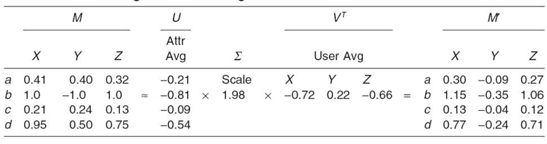
TABLE 23.5. A New U^', Σ^', and V^{T '} Produced from the Difference between M M^'

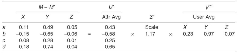
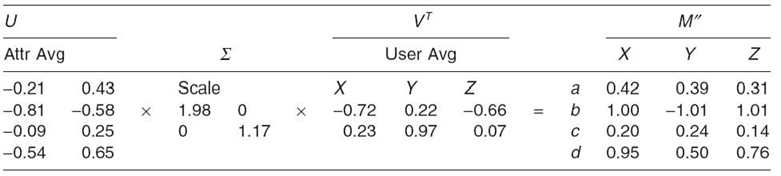
TABLE 23.6. M^" Produced from a More Complete U, Σ and V^T

While the estimated matrix, M^', in Table 23.4 is not identical to the original matrix, M, the relationships between the objects are maintained. X and Y are negatively related. X and Z are positively related. To correct for the error in the estimated matrix, the residual difference between the original and estimated matrices is used to calculate a new set of averages (U and V^T) and another scaling factor (Σ), The new matrices are shown in Table 23.5.

The original and new matrices (from Table 23.4 and 23.5, respectively) are concatenated to produce two columns as U and two rows as V^T. The new scaling factor is placed diagonally in a new ∑ Repeating the multiplication, a new matrix M^" is produced. Comparing Table 23.6 with Table 23.5 illustrates that M^" is significantly better than M^' as an estimate of M

The difference between this estimated matrix M^" and the original matrix M is used to create another matrix of residual values, which in turn are used to create another column of attribute averages in U, another scaling factor in ∑, and another row of user averages in V^T. The result is shown in Table 23.7.

TABLE 23.7. U, ∑, and V^T are Completed by Repeating the Decomposition Method on M-M^'

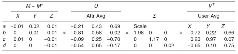
TABLE 23.8. Using ∑ to Estimate d for a New User T

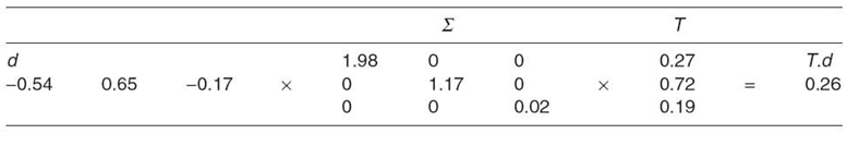
Table 23.7 depicts the SVD for the original matrix M. Attribute averages are represented by the U matrix. User averages are represented by the V^T matrix. The scale is represented by the ∑ matrix. Multiplied together, U ∑V^T = M. Further, the U and V^Tmatrices are not required to identify the relationships between the users and attributes. The ∑ matrix reflects composite information about the relationships between users and attributes. The U and V^T matrices contain information about specific attributes and users, not about relationships across the two sets. Since SVD is intended to store relationship information, only the diagonal values of the ∑ matrix are required. For this example, from Table 23.7, the user attribute relationship of M is represented by the vector {1.98, 1.17, 0.02}.

Once the SVD for existing data is calculated, it is possible to predict missing attributes for users. Assume a new user, T, is introduced. Only the first three attributes, a, b, and c, are known for this user. Using these three attributes, the user average column for T is calculated to be {0.27, 0.72, 0.19}. The value of the missing attribute, d, for T is estimated in Table 23.8.

By estimating missing attributes for users, it is possible to maintain accurate similarity measures among all users. Further, SVD is not affected by synonymy or polysemy. The KNN algorithm compares each attribute separately. Synonymy and polysemy artificially alter the weight of attributes. SVD produces a relationship value, ∑from all attributes for all users at the same time. Having a value repeated or two values combined in the attributes will result in U, ∑ and V^T matrices that produce the original matrix M with the same repeated or combined attributes.

23.3.3   Data Sparsity

Even with SVD, clustering is often difficult due to the sparsity of data [28]. The ability of a clustering algorithm to handle slight changes or omissions in data is often referred to as numerical stability. Without numerical stability, the overfitting of estimated or rounded values will likely be magnified in the final result [23]. Impuning missing values in sparse data without skewing the overall data set is important in many areas of statistical analysis [29].

Netflix has offered rewards for assistance in developing numerically stable algorithms for recommending movies to their customers. Due to the fact that most customers have relatively few movie selections (as compared to the number of movies available in the Netflix library), the Netflix data set is extremely sparse [30]. Calculating the SVD and then using it to accurately estimate missing data can be a time-consuming task.

The Lanczos algorithm was designed specifically as a method for calculating SVD [31]. It is an effective iterative algorithm for handling large but sparse data sets. Being iterative, the Lanczos algorithm will result in round-off error. Depending on implementation, it is possible to lose numerical stability. Three techniques to combat numerical instability when implementing the Lanczos algorithm are (1) preventing the loss of orthogonality, (2) recovering orthogonality after the basis is generated, and (3) removal of spurious eigenvalues after all eigenvalues have been identified [32].

The Lanczos algorithm is a simplified form of the Arnoldi algorithm [31]. As such, existing methods of implementing the Arnoldi algorithm are often used in place of the Lanczos algorithm. Due to computations that benefit from SVD in fluid dynamics, electrical engineering, and materials science, research continues to find methods of accelerating both the Lanczos and Arnoldi algorithms [33].

The overall issue of data sparsity is important for a predictive search engine. Consider the user-to-item ratio for Google. Google stores over one trillion (10¹²) unique URLs in their database [34]. With fewer than seven billion people in the world, each person could view 140 URLs, without any two people viewing the same URL. Further, even an avid web user will not have visited a significant percentage of the available URLs. As a result, Google users cannot be expected to have much user history in common. To compare and predict usage, most of the user data must be estimated.

In search engine usage, the user-to-item relationship is either “visited” or “not visited.” As such, search engine usage data are binary and estimation of user data is less complex than other estimation tasks, such as estimating how users might rate a movie or song. Many statistical techniques have been developed that successfully analyze sparse binary matrices using SVD [35]. These methods have been proven so effective that nonbinary data sets have been converted to binary data sets for quick estimation and analysis [30]. Therefore, binary SVD analysis will increase information and decrease sparsity by estimating what other items the user would likely select.

23.3.4  Grouping with SVD

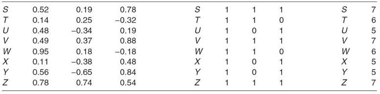
As demonstrated previously, SVD is commonly used for handling data synonymy, polysemy, and scarcity. Less commonly cited is another benefit of SVD, the ability to perform efficient and reliable similarity clustering [23, 36]. If the original matrix M is a mapping of customers to products, the matrices U and V^T, respectively, describe the customers and products with normalized values. Consider the example eight-customer matrix V (transposed from V^T) depicted in Table 23.9. First, each positive value is replaced with a “1.” Each negative value is replaced with a “0.” To make the result easier to read, the elements of each row are collectively read as a single binary number, which is then represented in decimal. As an example, theelements of row 1 of the middle matrix in Table 23.9, all three of which are binary “1,” are read as the binary number “111,” which is then represented as the decimal number “10.” The result of carrying out this operation on the customer matrix is a vector that represents each customer with one number. Customers with the same decimal number are in the same group. Customers S, V, and Z are in the same neighborhood of similarity. Customers U, X, and Y are in another neighborhood. If desired, the U matrix (produced from the original customer‒product matrix M)(see Table 23.1) could be used to easily group the products into neighborhoods of similarity.

TABLE 23.9. Producing Groups of Similarity for Eight Customers Using SVD

The benefit of using the same function to group all objects into neighborhoods of similarity is obvious, but it comes at a cost. SVD is a complex and time-consuming function. It does not allow for limiting the size of neighborhoods. Within a neighborhood, it does not indicate the relative similarity among objects. When speed, the ability to constrain the size of neighborhoods, or relative similarity are important, the KNN algorithm is preferred. Further, the SVD does not define what it means to be similar as it places customers into neighborhoods of similarity.

23.4   SIMILARITY METRICS

Accurate identification of similar (or different) objects is entirely contingent upon definition of a meaningful metric for similarity. There is no standard for a perfect measure of similarity. Consistency is one important consideration; given the same two objects, a similarity metric should always yield the same result. With rare exception, similarity metrics can be classified as either vector-or string based. Vector-based metrics treat data as a vector defined on a multidimensional space and compare the angle between vectors to determine similarity. String-based metrics treat data as ordered arrays of values and compare the elements of the arrays. Both categories of similarity metrics are examined in this section.

23.4.1   Vector-Based Similarity Metrics

Vector-based similarity metrics are common due to their simplicity of implementation and speed of calculation. The comparison between two vectors can be performed in linear time; that is, two objects with n attributes can be compared in O(n) time, compared with the O(n²) complexity of most string comparisons of n attributes. Consequently, vector-based similarity metrics are appropriate for objects with large attribute sets. For example, vector similarity is the standard method used in data mining to compare large volumes of text [37]; vectors represent frequencies of words found in the text. The result of a vector-based comparison will be “0” for completely dissimilar texts and “1” for identical texts.

TABLE 23.10. Genre of the Top Ten Movies of 2009, on a Scale of 0‒9

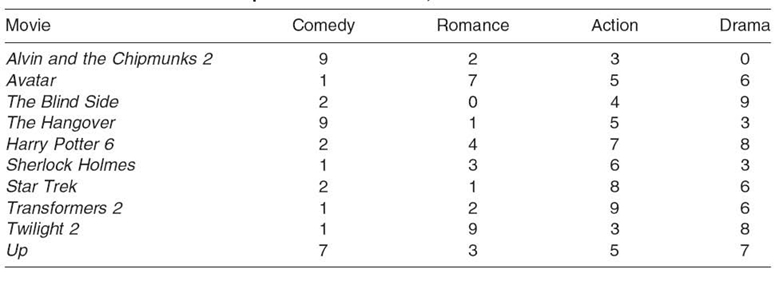
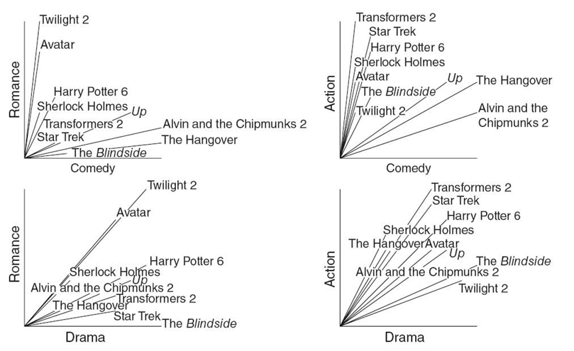
FIGURE 23.6. Attributes of the top 10 movies of 2009, plotted in four vector graphs.

The drawback to vector-based algorithms is the limitation of vector-based attributes. Given a large set of items, all items must be characterized using the same set of attributes. Each attribute becomes a dimension in the vector comparison. Table 23.10 is an example of using the attributes of comedy, romance, action, and drama to describe and compare the top 10 movies of 2009. Each attribute ranks the movie ´ s relevance to the particular genre from 0 to 9.

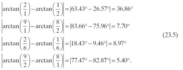
The purpose of vector-based similarity metrics is to calculate the angle between two vectors. The attribute vectors for each movie are plotted in Figure 23.6, with two attributes per graph. The angle between each pair of vectors is a measure of similarity. The smaller the angle between the two vectors, the more similar the corresponding movies.

Based on Figure 23.6, Alvin and the Chipmunks 2 appears to be similar to The Hangover; however, one is a children´s movie and the other is intended for adults. What is missing is a dimension that differentiates movies aimed at children from movies aimed at adults. The missing attribute leads to inaccurate vector similarity. Adding more attributes will increase the accuracy of vector similarity, at the cost of complexity in calculating the angles between all dimensions of the vectors. While some implementations, such as Amazon´s technique [15], aim for low dimensionality, others tolerate higher dimensionality, such as the Music Genome Project, which processes approximately 400 dimensions [22].

Examining Figure 23.6, it can be seen that the angles between Transformers 2 and Star Trek are relatively small. In the romance/comedy graph, Transformers 2 is at (1, 2) and Star Trek is at (2, 1). The angle between the vectors is 36.86°, as shown in the first line of the equation set (Equation 23.5). The average of all four angles is 14.73°, which is relatively small compared to the maximum possible, 90°:

23.4.1.1  Vector Cosine   Many common recommendation algorithms, such as the one implemented by Amazon, use vector cosine as a measure of similarity [15]. While maintaining reasonable accuracy, vector cosine is extremely fast compared to the trigonometric method (and the string-based methods of Section 23.4.2). Given two object attribute vectors, A and B, similarity is defined as the cosine of the angle between them. It is calculated with Equation (23.6), based on the “dot product” and “magnitude” vector operations. The dot product of two vectors is obtained by multiplying their corresponding elements, then adding the products to yield a scalar. The magnitude of a vector is the square root of the sum of the square of each element of the vector:

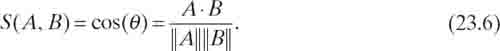
In the context of customer similarity, the attribute vectors A and B are usually a list of products purchased by customers A and B, respectively. For product similarity, the attribute vectors are usually a list of products purchased together. The resulting similarity is between −1, indicating polar opposition, to 1, indicating identity. A similarity value of 0 is commonly understood to be a sign of independence, indicating that the two objects have no relationship.

As an example, consider matrix M, in Table 23.11, where each object is represented by four attributes: a, b, c, and d, and attribute values are normalized between −1 and 1.

TABLE 23.11. Example of Normalized Attributes (a, b, c, and d) for Three Objects (X, Y, and Z)

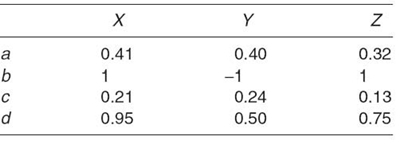
Using Equation (23.6), the similarity between X and Y is calculated in Equation (23.7):

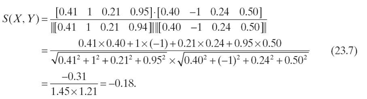
Likewise, the similarity between X and Z is 0.99, and the similarity between Y and Z is −0.3. It is not necessary to compare Y to X as the result will be the same as comparing X to Y due to the commutative property of the similarity function. Once all three vector cosines have been calculated, it can be stated that X and Z are most similar while X and Y are least similar.

With only three objects and four attributes, it is difficult to identify which object is most similar to X. Objects X and Y are most similar with respect to the a and b attributes. However, objects X and Z are most similar in the b and d attributes. Simply scanning data is not an effective means of comparing similarity. Vector cosine provides a method for producing a repeatable measurement of similarity. Increasing the number of attributes increases the computational complexity of determining similarity. In Equation (23.6), adding another attribute will increase the calculation by one multiplication and one addition in the numerator, and two squares and two additions in the denominator. In total, there will be an increase of three multiplications and three additions. With the addition of each attribute, the number of operations increases linearly—growing at a constant rate of three multiplications and three additions per attribute. Therefore, the complexity for vector cosine is bounded by O(n).

23.4.1.2   Vector Divergence   Vector cosine is a symmetric similarity metric, such that S (A, B) = S(B, A) for two vectors, A and B. Not all similarity metrics are symmetric. For example, if consumers tend to claim that Coke is similar to Pepsi, they should also make the symmetric claim that Pepsi is similar to Coke. In practice, the asymmetric claim that Pepsi is not similar to Coke persists [38]. A common asymmetric similarity metric is the Kullback-Leibler (KL) divergence. KL divergence is often used as a metric of difference, not similarity. More precisely, it is a measure of the difficulty of translating from one set of values (set A) to another (set B). The resulting value represents how many changes must be made to the original set (A) to attain the derived set (B). The greater the number of changes required, the more difficult the translation will be, indicating greater difference between sets A and B.

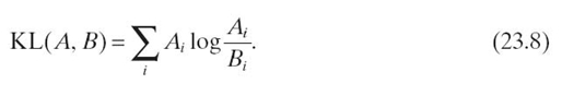
KL divergence is formally defined as in Equation (23.8), where each value A_i ∈ A is considered a measured value, and each value B_i ∈ B is considered an estimated value:

Comparing X and Z in matrix M (see Table 23.11), we can let the attributes of X be the reference set A. Then, the attributes of Z are the estimated set B. KL divergence produces a measure of difference between two sets of attributes (the greater the value, the greater the difference). As calculated in Equation (23.9), the difference between X and Z is 0.186. To make this value useful, it must be compared to a measurement between two other objects:

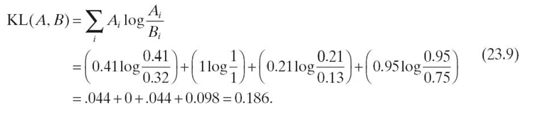
Of note, KL divergence could not be used to measure the difference between X and Y because attribute b would produce log(−1). This is a limitation of KL divergence.A_i and B_i must have the same sign. Taking the absolute value of A_i or B_i to make both positive would consider opposite values to be the same, creating an invalid comparision between A and B. Further, B_i cannot be zero. When A _i is zero, 0 log(0) is interpreted as zero [39]. If attribute b of X and Y is ignored (as doing so will not alter the KL divergence value for X and Z), the KL divergence value of X and Y would be 0.245. In other words, X and Y are more different from X and Z when attribute b is ignored, allowing KL divergence to be an alternative to vector cosine for data sets that meet the KL divergence constraints.

KL divergence is commonly used within LSI, a method that identifies patterns in relationships between sets of terms and sets of concepts in unstructured text [40, 41]. LSI has proven capable of overcoming two common hurdles in recommender system development. First, LSI easily handles synonymy. If two (or more) items in a data set are actually the same product, the items will be translated as identical vectors for analysis, making the synonymy obvious and easy to ignore. Second, LSI easily handles polysemy. If an item in a data set is actually more than one product, the item will be translated as a special vector for analysis that has the properties of each product that the item represents [42].

With recommender systems, LSI uses SVD to quickly calculate the KL divergence between a set of items and a set of customers. A problem in real-world implementations of LSI is that the divergence is calculated once. Over time, the divergence between items and customers may drift. A simple solution is to repeat the SVD/KL divergence calculation on a regular basis. Another solution is to approximate the drift in divergence as new information is gathered. This approximation is often referred to as ensemble learning, with variational divergence as a common form of ensemble learning [41]. With KL divergence, variational divergence is easy to estimate [40].

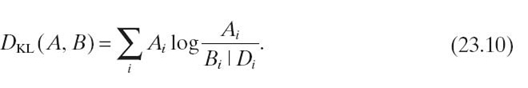
Given the standard KL divergence in Equation (23.8), the difference between the estimated relationship between A and B for a data set D is defined in Equation (23.10). Because this equation requires only an examination of the new data and the previously calculated SVD for A and B, it requires less time than a complete recalculation of the SVD:

Since the only bound on KL divergence is a lower bound of zero (no upper bound), repeatedly adjusting for new data may cause an incremental upward drift [40]. To avoid this possibility, it is helpful to calculate an upper bound that specifies a maximum level of difference. It is obvious that A is identical to itself and has a KL divergence of zero when compared to itself. Anything else that may be compared to A will have a difference greater than zero. When viewing the universe of possible sets, set A will be the origin. All other sets of information will be placed at varying distances away from the origin. At some point, there is a distance (or radius) away from the origin at which the information is deemed to be so different that further distinction between how different the information may be is meaningless. This information radius becomes the upper limit for KL divergence. Any values beyond the information radius are arbitrarily placed at the information radius.

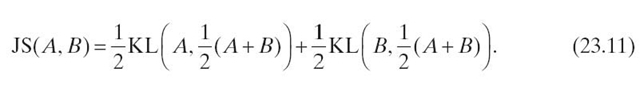
Jensen‒Shannon (JS) divergence may be used to calculate the aforementioned information radius [43]. Based on KL divergence, JS divergence has the useful addition of a finite result. In general, JS divergence, defined in Equation (23.11), is a symmetrized and smoothed version of KL divergence. Note that the equation for JS divergence makes two references to the equation for KL divergence. Therefore, the information radius comes at a cost of doubling the computation requirements:

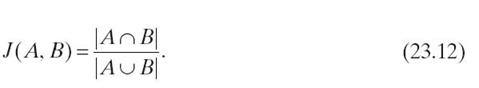
23.4.1.3   Variations on Vector Cosine   When attributes for an object have binary values, vector cosine may be simplified to the Jaccard similarity coefficient [44]. Given two sets of attributes, A and B, the Jaccard similarity coefficient is defined with the intersection and union operators (Equation 23.12). This results in a much faster operation than vector cosine (Equation 23.6). With n attributes, vector cosine will require about 3n multiplications and additions, along with two square root calculations. The Jaccard similarity coefficient is a counting function that can be performed with 2n additions and a division: First, count how many elements are in one of the sets by adding 1 to the count n times. (Because n is likely known beforehand, this count may not be necessary.) Then, count how many elements in each set are equal for the second set of addition. Divide the equal count by the size count to produce a Jaccard similarity:

The speed advantage of the Jaccard similarity coefficient comes with a slight loss of accuracy if vector cosine is considered a more correct metric of similarity. Consider two binary vectors, {1, 1, 0, 1} and {1, 0, 1, 1}. The vector cosine of the two vectors is 0.67. The Jaccard similarity coefficient of the two vectors is 0.50. It is difficult to see how Jaccard similarity coefficient and vector cosine relate to one another directly. However, the mathematical difference between the two is obvious when examining the Tanimoto coefficient [45].

If we limit all attribute values to binary 0 or 1, the Jaccard similarity and Tanimoto coefficients yield the same result [45]. The formula for the Tanimoto coefficient is defined in Equation (23.13):

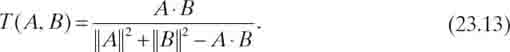
With the previous vectors {1, 1, 0, 1} and {1, 0, 1, 1}, the Jaccard similarity coefficient was 0.50. The Tanimoto coefficient is also 0.50. So, the Tanimoto coefficient shows how the Jaccard similarity coefficient may be written as a dot product and vector magnitude function, similar to vector cosine. The numerator is A·B in both functions, but the denominator of the Tanimoto coefficient is distinctly different from the denominator of the vector cosine. That produces a difference between the vector cosine and the Tanimoto coefficient (or Jaccard similarity). However, as with the vector cosine, the measure of similarity with either Jaccard or Tanimoto coefficients is simple and precise, allowing the Jaccard similarity coefficient to be a good option over vector cosine.

23.4.1.4   Similarity Indices   Vector cosines, along with Jaccard and Tanimoto, are often referred to as similarity coefficients, which are considered to be multiplicative factors of similarity. A coefficient of 0.50 implies similarity twice that of a coefficient of 0.25. Many other measures of similarity are referred to as indices. They are used for indexing items into clusters or groups of similarity. As such, a value of 0.50 does not necessarily reflect twice as much similarity as an index of 0.25. Unfortunately, the two terms are often used interchangeably, losing their meaning.

Many similarity indices come from the need to classify items, such as flowers, by similarity. Biological sciences have produced the most commonly used similarity indices, such as the Jaccard similarity coefficient and the S Ørensen index. Given two binary sets, the S Ørensen index (which also happens to be the definition of Dice´s coefficient) is identical to twice the Jaccard similarity coefficient. The common equation for both the S Ørensen index and the Dice coefficient is shown in Equation (23.14) [46, 47]:

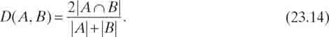
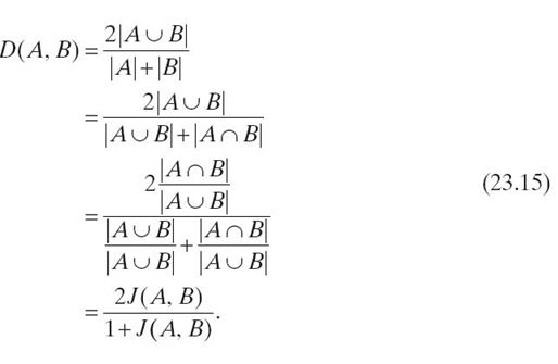
The only issue in calculating Equation (23.14) is interpretation of | A ⋃ B | and | A | + | B |. For binary sets, some interpretations opt to omit zeros from | A ⋃ B |. If zeros are maintained, the number of items in the union of A and B is the same as the number of items in A added to the number of items in B. However, a purely mathematical view of | A | + | B | would consider it equal to | A ⋃ B |. If that is the case, Dice´s coefficient is related to the Jaccard similarity coefficient by Equation (23.15):

Within the scope of comparing the expansive search history of multiple users, similarity metrics that are based solely on union and intersection operators will require fewer operations on a computer than vector cosine. Further, because set operations are dependent on counting, specialized incrementers may be used in place of standard adders. Both up and down counters can be implemented to run much faster than an adder [48].

23.4.1.5   Limitation of Similarity   As mentioned in Section 23.3, a common experience that most users have with similarity measures is Amazon´s recommendation system. Each customer is categorized by the products that he or she has purchased. SVD and vector cosine are used to place customers into similarity neighborhoods. Amazon then recommends products to each customer based on the products purchased by others in the same similarity neighborhood [15].

This is effective in defining which products, collectively, groups of customers are purchasing. It also helps identify products that tend to be purchased together. However, this method is greatly limited by the loss of order. Amazon does not suggest which products should be purchased next. The sequence in which purchases were made is not considered in making a recommendation.

Consider a book series, such as the Harry Potter series. After purchasing Book 5 in the series, Amazon will suggest purchasing Books 1, 2, 3, and 4. However, it is highly unlikely that many people purchase book 5 in a series without having already read the previous four books. If order was taken into account, Amazon may suggest purchasing Books 6 and 7 and ignore the previous books.

Vector-based comparisons consider all attributes as dimensions. Without any priority order among attributes, no dimension comes before another dimension. Values within a dimension are not time ordered. The lack of order leads to a very fast calculation of similarity, but a loss of time-ordered relevance. A comparison that keeps events, such as books ordered by customers, in order would be preferable for a recommendation system, especially a search engine recommendation system. Users are interested in seeing which search results come next, not search results that may have been visited in the past.

23.4.1.6   Summary of Vector Comparison Algorithms   Vector comparison algorithms are based on the observation that when objects are represented as vectors originating at the origin, the angle between the vectors is smaller when the objects are similar and larger when the objects are different. The angle is commonly measured with the vector cosine equation. With many multiplications and square root functions, the vector cosine equation can be considered complex. Simpler functions exist that produce equivalent results when the attributes are represented as binary values. Because much of the data used in real-world applications are binary, it is common to find the Jaccard similarity coefficient or the S Ørensen index used in place of the vector cosine. Both of the former are based on union and intersection functions, which are implemented as simple counting functions. By using the Tanimoto coefficient as a reference, it is possible to see how the union and intersection functions may be rewritten as dot product and vector magnitude functions, similar to vector cosine, which demonstrates the validity of using the simpler coefficients in place of vector cosine.

23.4.2   String-Based Comparison Algorithms

If events are time ordered and can be represented symbolically, it is possible to treat a sequence of events as an ordered set or a string. There are many orde-preserving algorithms for comparing two strings [19, 49]. For the most part, these algorithms descend from Hamming distance, which directly relates to vector-based similarity.

Hamming distance is a measure of the number of positions in which two strings have different symbols [50]. The two binary strings, “1011001” and “1001101,” have a Hamming distance of two because they differ in two positions (bits three and five). This type of measurement is nearly identical to the Jaccard coefficient (and the related Tanimoto, S Ørensen, and Dice measurements).

If each position is considered as an attribute, the first string is the set {1, 0, 1, 1, 0, 0, 1} and the second string is the set {1, 0, 0, 1, 1, 0, 1}. The two sets share five of the seven attributes considered. The Jaccard coefficient is calculated as in Equation (23.16):

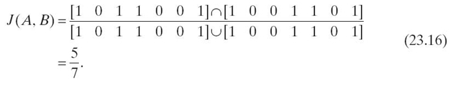
Note that the application of Hamming distance is limited to strings of equal length. Therefore, the denominator used to account for sets of different lengths in the Jaccard coefficient would be the same value for all comparisons when all strings have equal length. Being redundant, the denominator is not needed in the Hamming distance. If the denominator of the Jaccard coefficient is removed, the Hamming distance is the length of either string minus the Jaccard coefficient. In other words, the Jaccard coefficient is a measure of similarity and the Hamming distance is a measure of difference.

23.4.2.1   Converting Difference to Similarity   String-based comparison algorithms tend to measure the distance (or difference) between two strings. They do not measure similarity. Two identical strings will have absolutely no difference. From there, the difference grows as a distance from being identical. Because there is no universal measure of absolute difference, distance from being identical is a reasonable measure.

To convert difference to similarity, the maximum difference must be known. A distance of zero indicates identical strings. If the maximum difference between two strings is M, the range between being identical and being completely different is known. Similarity may be calculated as shown in Equation (23.17):

If the distance is 0, similarity will be 100 %. If the distance is M, similarity will be 0 %. While this is an effective method for converting difference to similarity, it has limitations dependent on the algorithms used to measure difference.

Consider an application that attempts to match unknown words to a dictionary of known words. Using a string difference algorithm (the specific algorithm is not important in this example), the word “busnes” is compared to “busses” and “business.” The algorithm calculates the difference for both comparisons to be 2. For this algorithm, assume that the maximum possible difference is the length of the longest string among the strings being compared. Converting to similarity, busnes is (6−2)/6 = 0.67 similar to busses and (8−2)/8 = 0.75 similar to business. While the difference is the same for both strings, the conversion to similarity clearly gives precedence to longer strings when making comparisons.

23.4.2.2   Levenshtein Distance   Most string-based distance measurements are based on Levenshtein distance, an extension of Hamming distance [51]. It removes the limitation of a binary alphabet, allowing for an alphabet of any arbitrary size. It also removes the limitation that the two strings must be of equal length. In doing so, Levenshtein distance measures three differences between the two strings being compared:

• Insertion. The difference between “cat” and “coat” is an insertion of “o.”
• Deletion. The difference between “link” and “ink” is a deletion of “l.”
• Substitution. The difference between “lunch” and “lurch” is the substitution of “r” for “n.”

Each difference is counted. The total number of differences is the Levenshtein distance between the two strings. For example, the Levenshtein distance between “Sunday” and “Saturday” is three: an insertion of “a,” an insertion of “t,” and a substitution of “r” for “n.”

23.4.2.3   Calculating L evenshtein Distance   As an optimization problem over two arbitrary length strings, calculating Levenshtein distance is a common example used in dynamic programming [52, 53]. The Wagner‒Fischer algorithm is a dynamic programming method for calculating Levenshtein distance. Given two strings of respectively, the runtime of the Wagner‒Fischer algorithm is O(mn) [54]. A typical recursive solution requires O(mn²).

TABLE 23.12. Initializing a Matrix for the Wagner‒Fischer Algorithm

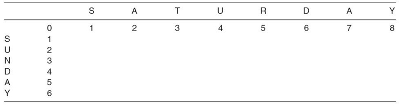
TABLE 23.13. Completed Matrix for the Wagner‒Fischer Algorithm

The Wagner‒Fischer algorithm is a matrix solution for two strings, A and B. For strings A and B of length m and n, respectively, an (m + 1) × (n + 1) matrix is created. The top row of the matrix is filled with increasing integers 0, 1, 2, 3…from left to right. Similarly, the leftmost column is populated with increasing integers from top to bottom. For comparing “SUNDAY” (string A) to “SATURDAY” (string B), the initial matrix is shown in Table 23.12.

With the initial matrix setup, each of its elements is filled in, from top to bottom and left to right, according to Equation (23.18):

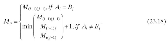
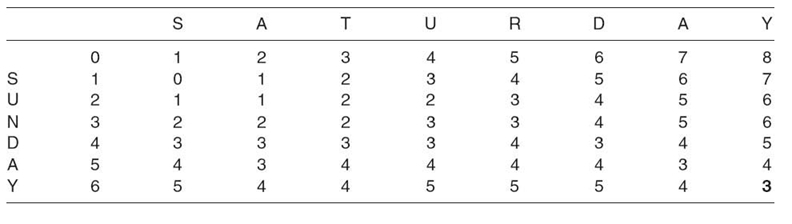
For example, as “S” equals “S” in the first element to fill in, M_{1, 1} is set to zero. S in SUNDAY does not match “A” in SATURDAY; hence, M_{1, 2} gets the value min(1, 2, 0) + 1, which is 1. After completing all elements, the matrix will contain the values shown in Table 23.13.

When completed, the value in the bottom right corner is the Levenshtein distance between the two strings. For SUNDAY and SATURDAY, the distance is three. Because the maximum Levenshtein distance is the length of the longest string (8 in this example), the similarity would be (8−3)/8 or 62.5 %. This value is comparable to that of vector-based measures of similarity: Jaccard coefficient = 5/8 = 62.5 % Dice´s coefficient = 2 × 5/(6 + 7) = 76.9 %.

Consider changing the order of the characters in the strings. Doing so does not change the vector-based measures. Each character is an attribute without order. From a string-based comparison, “DAYSUN” and “SATURDAY” have a difference of 7, which is a similarity of (8−7)/8 = 12.5 %.

For comparison of search engine usage, Levenshtein distance accurately indicates the ordered difference between users because the order in which the search results are selected is maintained. A user with a history of {A, B, C, D} will be considered very different from a user with a history of {D, C, B, A} with a string-based comparison, while a vector-based comparison will show that the two users selected the same results.

As noted previously, converting difference to similarity can produce undesirable results due to the varying length of strings being compared. Levenshtein distance is unreliable at comparing short strings to extremely long strings. What if one user has a history of {A, B, C}, and another user with a search history containing over 100 items also has visited A, B, and C, in the same order? Further, what if many users have visited A, B, D, C, in that specific order? Identifying this common behavior is important to predicting overall search engine use. A method of finding out if a short string is nearly a substring of a long string is necessary.

23.4.2.4  String Alignment   Given two strings, A and B, a common task that is related to testing for similarity is the task of alignment. Assuming that A is shorter in length than B, the goal is to alter A in order to maximize similarity (minimize difference) of A compared to B. There are two forms of string alignment: global and local.

Global alignment will add gaps (a special null symbol) to A, increasing the length of A to the same length as B. While doing so, the difference between A and B is minimized.

Local alignment not only alters A but it also identifies a substring of B for which the substring and the altered A have the minimum distance. This is technically a global alignment between A and a substring of B.

For global alignment and local alignment, the Needleman‒Wunsch algorithm [55] and the Smith‒Waterman algorithm [51] are commonly used, respectively. Both are slight adaptations of the Wagner‒Fischer algorithm.

23.4.2.5   Global Alignment: Needleman‒Wunsch Algorithm   The Needleman‒Wunsch algorithm is a matrix solution [55]. Given two strings, A and B, of length m and n, respectively, an (m + 1) × (n + 1) matrix M is created. Traditionally, the shorter string is placed from top to bottom along the left side of the matrix. The longer string is placed from left to right along the top of the matrix.

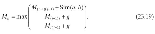
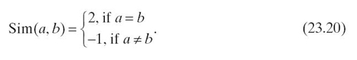
Similar to the Wagner‒Fischer algorithm, each cell of the matrix is filled according to Equation (23.19). The Needleman‒Wunsch algorithm adds a gap penalty, g, which helps place gaps in A such that the difference between A and B is minimized. The value of the gap penalty depends on the application and the desired result. Also, it is popular to use a similarity matrix to weight different comparisons between a and b (elements of A and B, respectively). This is indicated in Equation (23.19) as the function Sim. An example similarity matrix is shown in Table 23.14. Using this similarity matrix, if a = G and b = C, the similarity is −5. It is possible to replace the similarity matrix with a similarity function that performs a mathematical calculation on the values of a and b. In the case of Levenshtein distance, the similarity function produces 0 when a = b and 1 otherwise:

TABLE 23.14. An Example Similarity Matrix forComparing DNA Sequences

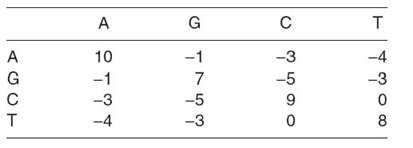
TABLE 23.15. Initializing a Table for the Needleman‒Wunsch Algorithm

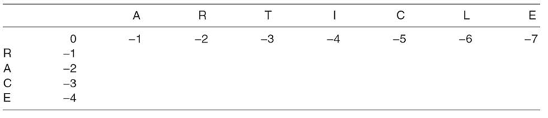
TABLE 23.16. A Completed Table for the Needleman‒Wunsch Algorithm

Before filling in the cells of M, the top row and left column are initialized with values based on the gap penalty. For rows i = 0 to m, M_{(i, 0)}is filled with g × i, where g is the gap penalty. For columns j = 0 to n, M_{(0, j)} is filled with g×j. Using a gap penalty of −1 to compare “RACE” to “ARTICLE,” the initialized matrix is shown in Table 23.15.

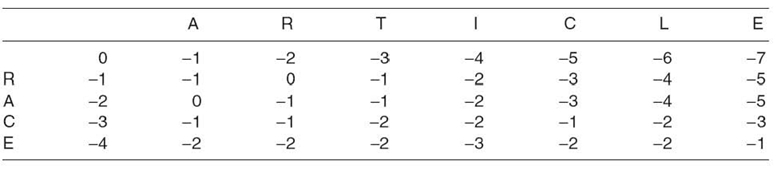
For columns j = 1 to n in row i = 1 each cell M_{i, j} is filled by comparing a to b with Equation(23.19). Unlike the Wagner‒Fischer algorithm, the Needleman‒Wunsch algorithm lowers values for a mismatch. Table 23.16 is a completed matrix where Sim(a, b) is set to “1” on equality and “− 1” on inequality. The gap penalty g, is “− 1.”

After completing the matrix, global alignment is discovered by backtracking from the lower right corner to the upper left corner. For each cell, the direction to the neighbor with the largest value is indicated. Only three neighboring cells are compared: the cells above, above to the left, and to the left. When more than one cell contains the greatest value, the indicator can point to either. Table 23.17 includes arrows indicating the neighbor with the greatest value.

TABLE 23.17. A Completed Needleman‒Wunsch Table with Backtracking Arrows

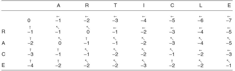
The best global alignment is calculated by following the arrows from the lower right corner of Table 23.17 to the upper left corner. When in a cell in which the symbol of A matches the symbol of B for the cell, write down the symbol. If the symbol of A does not match the symbol of B, write a gap symbol. When complete, the aligned A will be “‒R‒‒C‒E”: a string that is the same length as B with minimum distance.

With this example, it may be shown that global alignment is also useful for identifying a common path. Assume that ARTICLE is a set of seven ordered locations, such as websites or street intersections, each identified by a letter. Then, assume that RACE is another set of four ordered locations. After creating a global alignment,‒R‒‒C‒E is produced. The common path between ARTICLE and RACE is “RCE,” in that specific order. Even though both sets contain the location “A,” it is not part of the global alignment and, therefore, not part of the common path.

23.4.2.6   Local Alignment: Smith‒Waterman Algorithm   The Smith‒Waterman algorithm is yet another adaptation of the same matrix solution used in the algorithms previously discussed in Section 23.4.2.3 and 23.4.2.5. With strings A and B, of lengths m and n, respectively, a matrix M of size (m + 1) × (n + 1) is created. All cells in the top row and left column of M are initialized to zero. The similarity function is similar to the Needleman‒Wunsch algorithm. In this example, the similarity function is given in Equation (23.20):

Where as the Needleman‒Wunsch algorithm had a single gap penalty, the Smith‒Waterman algorithm has both a deletion (p_d) and an insertion (p_i) penalty. If p_d = p_i, it is essentially equivalent to a single gap penalty. Separating the gap penalty into two penalties allows the implementation to add extra weight to either deletions or insertions. For simplicity, the following example will use −1 for both p_d and p_i.

After the top row and left column are initialized to zero, the rest of the matrix is populated. Similar to the Wagner‒Fischer and Needleman‒Wunsch algorithms, the cells are filled in from the top left to the bottom right, using Equation (23.21): It is important to note that including the zero in values compared by the max function eliminates the possibility of a negative value in any cell of the matrix. Therefore, the cells that contain nonzero values will be those cells in which a match has generated an increase in value from the neighboring cells. An example that compares “BELL” to “UMBRELLA” is shown in Table 23.18.

TABLE 23.18. A Completed Smith‒Waterman Matrix

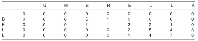
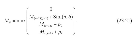
It is important to note that including the zero in values compared by the max function eliminates the possibility of a negative value in any cell of the matrix. Therefore, the cells that contain nonzero values will be those cells in which a match has generated an increase in value from the neighboring cells. An example that compares “BELL” to “UMBRELLA” is shown in Table 23.18.

To locate the local alignment of a completed Smith‒Waterman matrix, the cell with the greatest value is located (the cell with a value of 7 in the example in Table 23.18). From the current cell, the neighboring cell (up, up/left, or left) that contains the greatest value is located. This continues until all neighboring cells contain a zero. In this example, the best alignment begins at the cell containing a 7, continues up/left to a 5, up/left to a 3, then either left or up/left to a 1, and finally to the cell containing a 2. When the symbols in both strings match, write the symbol. A gap symbol is used otherwise. The local alignment of BELL to UMBRELLA is “B-ELL.”

Local alignment is a useful tool for identifying the part of a long sequence that is a good match for a short sequence. For example, assume that a customer´s last four purchases are known, each item identified by a letter to be BELL. To locate trends, the complete purchase history of other customers will be searched for the same sequence of items. Instead of limiting the search specifically to BELL, local alignment allows for a search of subsequences that are very similar, such as “BRELL.” As such, the number of matching search histories will likely be larger than the number that contains BELL without alteration.

23.4.2.7   Wagner‒Fischer Complexity Improvements   The primary reason that the Wagner‒Fischer and related algorithms are not commonly used is their high complexity. For strings of length m and n, the complexity is bounded by O(mn). Methods of addressing the complexity challenge of the Wagner‒Fischer algorithm include the following:

• By maintaining the values of only two rows at a time, the space required in memory is reduced from mn to 2m. This decreases memory requirement. In the case of large values of m and n, reducing memory requirement may reduce memory swapping, which in turn may reduce total execution time.
• If the only interest is in detecting a difference that exceeds a threshold k, then it is only necessary to calculate a diagonal stripe of width 2k + 1. The complexity becomes O(kn), which is faster whenever k < m [ 49, 56].
• Using lazy evaluation on the diagonals instead of rows, the complexity becomes O(m(1 + d)), where d is the calculated Levenshtein distance. When the distance is small, this is a significant improvement [57].

Estimation is a popular method applied to calculating global and local alignments in DNA sequences. Two algorithms have been developed: BLAST and FASTA. BLAST greatly reduces the execution time of the Smith‒Waterman algorithm by first estimating a match against a subset of a DNA database and then comparing groups of positions, usually three at a time [58]. FASTA operates in the same manner, using a different heuristic for estimating the initial match against a subset of a DNA database [56].

To apply either of these approaches to comparing search engine results, a database of common sequences of results must be created. When there are many users over a relatively small set of possible results, it will be expected that specific sequences of three or four search results will occur frequently. However, many search engines have very few users compared to the set of possible results. Consequently, the odds of having a high number of repeated sequences of search results drop significantly. Further, calculating the longest and most common sequences of results in a data set is time-consuming. Such calculations are very similar to the task of identifying common sequences of bytes in a file when executing common file compression algorithms, such as bzip2 or LZMA. Assume that the search results to be checked will not be presorted by frequency of occurrence or selection. The expected complexity of most common compression algorithms will be O(n log n), where n is the total number of search result selections across all users being compared [59].

Assuming that a compression method is implemented, a new problem arises. If the sequence of results (“A,” “B,” “C”) is encoded with “1” and the sequence (“A,” “C”) is encoded with “2,” it is no longer possible to compare 1 to 2 and detect matching characters. Instead, a similarity matrix must be created that compares all encodings to one another. In this case, 1 is 2/3 similar to 2. The complexity of generating the similarity matrix will be at least O(n²) for n encodings.

An alternative that nearly matches the benefits of BLAST is to create a simple k-length dictionary from string B when comparing the two strings A and B. The dictionary is simply a list of all k-length substrings in B. For the string UMBRELLA and k = 3, the dictionary contains “UMB,” “MBR,” “BRE,” and so on. Instead of searching A for sequences in a database, each substring in the dictionary is compared to A. If A is BELL, the only matching substring is “ELL.” Then, an attempt is made to expand the match. Because both UMBRELLA and BELL contain a “B” before “ELL,” the match is expanded to include “B” with a gap. The resulting local alignment is “B-ELL.” Increasing the value of k will decrease the execution time by decreasing the number of substrings in the dictionary. However, higher values of k decrease sensitivity in locating small local alignment. For example, with k = 4, there is no match between BELL and UMBRELLA.

A similar method of comparing two strings in smaller sections was proposed by Monge and Elkan [60]. If the strings of data to be compared can be logically reduced to distinct substrings, such as dividing full names into first, middle, and last names, then each substring pair is compared in place of the overall comparison. For example, comparing “John Paul Jones” to “Jones, John P.” directly would require 15 × 14 = 210 steps. The string “John Paul Jones” is obviously a concatenation of the substrings “John,” “Paul,” and “Jones.” Sorted, they become the set (“Paul,” “John,” “Jones”). The string “Jones, John P.” becomes the sorted set (“P.,” “John,” “Jones”).(The punctuation could be omitted but is retained in this example for a worst-case scenario.) In the Monge‒Elkan algorithm, “Paul” is compared to “P.” in 4 × 2 = 8 steps, “John” is compared to “John” in 4 × 4 = 16 steps, and “Jones” is compared to “Jones,” in 5 × 6 = 30 steps. The total number of steps is 8 + 16 + 30 = 54, an improvement of 74 %. Unfortunately, the requirement of logical and sortable substrings greatly limits the benefit of the Monge‒Elkan algorithm.

23.4.2.8   Summary of String Comparison Algorithms   The strong relationship between the Jaccard similarity coefficient and Hamming distance makes it evident that vector-based and string-based comparison algorithms are similar. The difference between the two is order. Given three attributes, such as A, B, and C, vector-based algorithms will consider only the value of each attribute. String-based algorithms will consider the order in which an object implements each of the attributes, along with the attribute´s value.

Three very common forms of string-based algorithms are Levenshtein distance, Needleman‒Wunsch distance, and Smith‒Waterman distance. All are commonly implemented through adaptations of the Wagner‒Fischer matrix-based dynamic programming solution. Levenshtein distance is used to identify the distance between two strings of data. Needleman‒Wunsch distance is used to identify distance while adding gaps to the shorter string to produce two strings that are of the same length and have minimal distance. This is referred to as global alignment. Local alignment, by contrast, aligns the shorter string with a substring of the longer string of data. Smith‒Waterman distance provides local alignment.

Because of the complexity involved in calculating string-based comparisons, many shortcuts have been developed. Within the realm of DNA comparison and sequencing, BLAST and FASTA have been used to estimate alignment with a dictionary of common sequence comparisons. It is difficult to produce a similar dictionary for data where the range of values vastly exceed the four DNA values of a, g, t, and c. One solution is to divide strings of data into logical substrings and then to compare the substrings with one another, as in the Monge‒Elkan algorithm. When this division is feasible, the resulting improvement in complexity is significant. However, it is often difficult to define logical substrings in real data. Therefore, string-based comparison algorithms tend to be used only when order is vital to the overall task. Otherwise, vector-based algorithms are implemented.

23.5   CONCLUSION AND FUTURE WORK

The goal of this research is to use historical data for all users of a search engine to predict which search results a specific user will likely select in the future. This can be accomplished by developing a behavior model to predict user behavior. To improve the accuracy of the predictions, the users should be separated into neighborhoods of similarity based primarily on previous search engine usage. Other user information, such as locale or gender, may be used for similarity comparisons. A behavior model is then generated for each neighborhood.

Grouping users into neighborhoods is a general concept, with many options. Each user´s history, as well as any known information about the users, must be normalized into a distinct set of user attributes. Given a matrix of users and attributes, it is possible to compare users for similarity. However, it is expected that the matrix will suffer from sparsity, synonymy, and polysemy. Data correction through the use of SVD should limit all three issues. SVD can be implemented quickly with either Lanczos or Arnoldi iterative algorithms. If limited to binary data, binary SVD algorithms have been noted for accurate estimation in sparse binary data sets.

Once data correction is complete, comparison of users could be a simple vector comparison or a complex string comparison. Within the realm of vector comparisons, vector cosine is an efficient method of identifying similarity between two users. Within the realm of string comparisons, Levenshtein distance is a more accurate measure of differences in the history of each user. Vector cosine executes within a bound of O(n). Levenshtein has complexity of O(n²).

In choosing between a vector or string comparison, computational complexity is not the only issue to consider. A vector comparison will identify users who have selected similar search results in the past, regardless of the order in which those results were selected. A string-based comparison considers the order and, depending on the algorithm used, aligns users such that similarity of history is considered while ignoring divergence of history.

Grouping users into neighborhoods and identifying behavior models are two distinctly different steps in the process of designing a predictive search engine. As such, it is reasonable to implement both vector-based comparisons and string-based comparisons as needed. Vector-based comparisons will be significantly faster when grouping users into neighborhoods of similarity. Once grouped, string-based comparisons will be useful in aligning user search histories and in developing a user behavior model for the group.

The success of this predictive method can be tested by gathering usage logs from multiple search engines. Grouping the users into neighborhoods of similarity should be validated first. A user behavior model should then be developed for each group. The goal is to have a usage model that, given the sequence of search items previously selected, has a very high probability of successfully predicting the search items that the users within the neighborhood will select next. If successfully and correctly implemented, this predictive search method can considerably reduce total search time. As an additional benefit, the method can direct a user to a sequence of resources that are popular within the user´s similarity neighborhood.

 

Appendix A

Comparative Analysis of Comparison Algorithms

Table A.1 is a comparison of the popular comparison algorithms described in this chapter. For all algorithms, the sets being compared are referred to as A and B. Each set consists of independent data items, m items in A and n items in B. Limitations on the types of data items allowed are indicated for each algorithm. For example, Hamming distance is limited to binary data. Complexity is directly related to estimated execution time. Complexity is shown with trivial cases here for comparison. For example, (mn) is slightly less complex than (mn + n), though both are O(mn). Some algorithms work with elements in groups. In such cases, the group size is represented as c. The minimum, maximum, and distribution of values are shown.

Table A.1 A Comparison of Comparison Algorithms

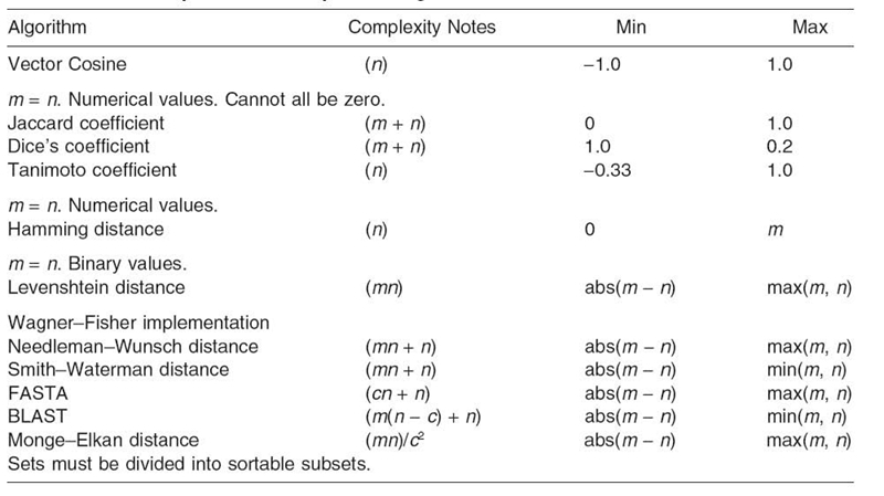
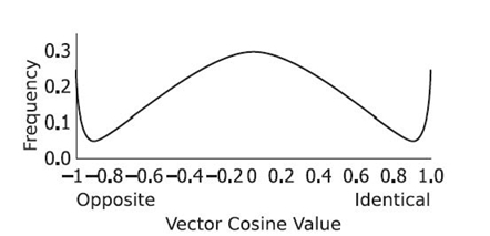
FIGURE A.1. Distribution of vector cosine values for 1,000,000 random sets.

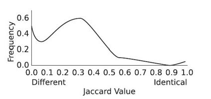
FIGURE A.2. Distribution of Jaccard coefficient values for 1,000,000 random sets.

Most comparison metrics do not produce a linear distribution of results from the minimum to maximum value. To plot an expected distribution, each metric was calculated for 1,000,000 random set pairs A and B. The results were plotted by frequency (normalized by dividing each frequency count by the square root of the square of all frequency counts). When using real-world data, the distribution will likely be different due to the expected bias of the real-world data compared to purely random data (Figs. A.1‒A.8).

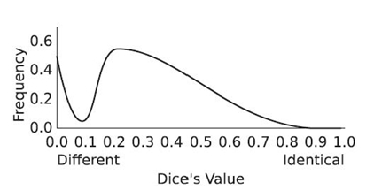
FIGURE A.3. Distribution of Dice´s coefficient values for 1,000,000 random sets.

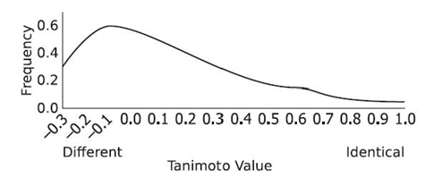
FIGURE A.4. Distribution of Tanimoto coeffi cient values for 1,000,000 random sets.

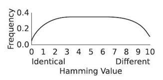
FIGURE A.5. Distribution of Hamming distance values for 1,000,000 random sets.

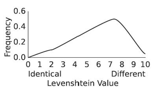
FIGURE A.6. Distribution of Levenshtein distance values for 1,000,000 random sets.

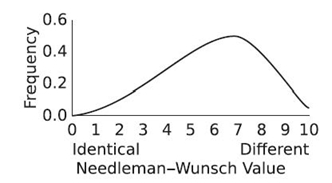
FIGURE A.7. Distribution of Needleman‒Wunsch distance values for 1,000,000 random sets.

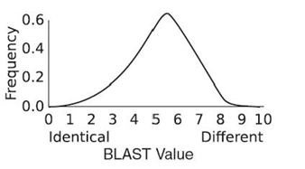
FIGURE A.8. Distribution of BLAST distance values for 1,000,000 random sets.

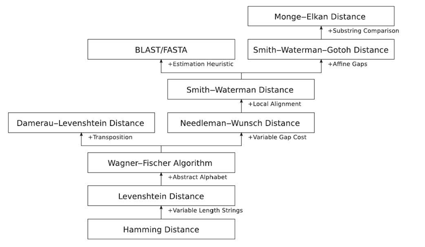
FIGURE A.9. Evolution of string-based comparison algorithms.

A.1   VECTOR-BASED COMPARISONS

For two sets A and B, the common vector-based comparison metrics are listed in Equations A.1‒A.4:

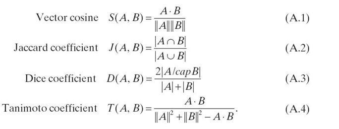
Appendix A.2   STRING-BASED COMPARISONS

The evolution of common string-based comparison metrics, from Hamming distance to modern algorithms, is shown in Figure A.9.

 

Appendix B

Most Popular Searches

Search engine traffic usage is tracked by Experian Hitwise (http://hitwise.com). Based on 4 weeks of usage (shown in Table B.1), the top five keyword searches comprise approximately 5 % of all searches.

Table B.1 Top Search Terms for Four Weeks Ending March 27, 2010

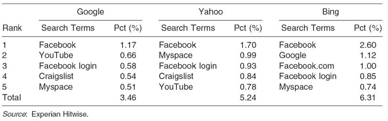
Based on this knowledge, if a search engine designer wished to decrease the load on the query processor by 5 %, he or she should simply cache the top five queries. As a result, if a user were to perform a query for Facebook or Myspace, the search engine would not process the query in a normal manner. It would recognize the query as one of the popular queries and would simply pull the results from cache.

Keeping a running list of which searches are most popular is not difficult. Many algorithms exist for keeping track of most popular events over time without allowing for past popular events to overshadow new events [61].

REFERENCES

[1] A. Rangaswamy, C.L. Giles, and S. Seres, “A strategic perspective on search engines: Thought candies for practitioners and researchers,” Journal of Interactive Marketing, 23(1): 49‒60, 2009.

[2] D. Hawking, N. Craswell, P. Brailey, and K. Griffihs, “Measuring search engine quality,” Information Retrieval, 4(1): 33‒59, 2001.

[3] M. Levene, An Introduction to Search Engines and Web Navigation. Hoboken, NJ: John Wiley & Sons, 2010. 2 ed.

[4] D. Lewandowski, “Search engine user behaviour: How can users be guided to quality content?” Information Services and Use, 28(3‒4): 261‒268, 2008.

[5] D. Tumer, M.A. Shah, and Y. Bitirim, “An empirical evaluation on semantic search performance of keyword-based and semantic search engines: Google, Yahoo, msn and Hakia,” in Proceedings of the 2009 4th International Conference on Internet Monitoring and Protection, pp. 51‒55, IEEE Computer Society, 2009.

[6] W.A. Wickelgren, “Speed-accuracy trade-off and information processing dynamics,”Acta Psychologica, 41 (1): 67‒85, 1977.

[7] Q. Gan and T. Suel, “Improved techniques for result caching in web search engines,” in Proceedings of the 18th International Conference on World Wide Web, WWW ´09, pp. 431‒440, ACM, 2009.

[8] R. Ozcan, I.S. Altingovde, B.B. Cambazoglu, F.P. Junqueira, and Õ. Ulusoy, “A five-level static cache architecture for web search engines,” Information Processing & Management, 47(2): 147‒308, 2011.

[9] L.A. Adamic, “The small world web,” in Proceedings of the 3rd European Conference on Research and Advanced Technology for Digital Libraries, ECDL ´99, pp. 443‒452, Springer-Verlag, 1999.

[10] About google instant. Available at http://www.google.com/instant/, November 2010.

[11] N.Y. Yen, T.K. Shih, L.R. Chao, and Q. Jin, “Ranking metrics and search guidance for learning object repository,” IEEE Transactions on Learning Technologies, 3(3): 250‒264, 2010.

[12] B.F. Skinner, The Behavior of Organisms. Acton, MA: Copley Publishing Group, 1938.

[13] T. Toledo and R. Katz, “State dependence in lane-changing models,” Transportation Research Record: Journal of the Transportation Research Board, 2124: 81‒88, 2009.

[14] A. Pentland and A. Liu, “Modeling and prediction of human behavior,” Neural Computation, 11(1): 229‒242, 1999.

[15] G. Linden, B. Smith, and J. York, “Amazon.com recommendations: Item-to-item collaborative filtering,” IEEE Internet Computing, 7(1): 76‒80, 2003.

[16] M.T. Jones, B. McClendon, A.P. Charaniya, and M. Ashbridge, “Entity display priority in a distributed geographic information system.” Available at http://www.google.com/patents/about?id = ZVepAAAAEBAJ &dq = patent: 7278103, June 2007.

[17] S. Cleger-Tamayo, J.M. Fern ández-Luna, J.F. Huete, R. P érez-V ázquez, and J.C. Rodr íguez Cano, “A proposal for news recommendation based on clustering techniques,” in Trends in Applied Intelligent Systems (N. Garc ía-Pedrajas, F. Herrera, C. Fyfe, J. Manuel Ben ítez, and M. Ali, eds.), Vol.6098 of Lecture Notes in Computer Science, pp. 478‒487. Berlin/Heidelberg: Springer, 2010.

[18] T.M. Cover and P.E. Hart, “Nearest neighbor pattern classification,” IEEE Transactions on Information Theory, 13(1): 21‒27, 1967.

[19] R. Xu and D.C. Wunsch II, “Survey of clustering algorithms,” Neural Networks, 16(3): 645‒678, 2005.

[20] M. Mukiibi and J.O. Bukenya, “Segmentation analysis of grocery shoppers in alabama,” in The Southern Agricultural Economics Association Annual Meeting, February 2008.

[21] D. Bremner, E. Demaine, J. Erickson, J. Iacono, S. Langeman, P. Morin, and G. Toussaint, “Output-sensitive algorithms for computing nearest - neighbour decision boundaries,”Discrete & Computational Geometry, 33(4): 593‒604, 2005.

[22] J. John, “Pandora and the Music Genome Project,” Scientific Computing, 23(10): 40‒41, 2006.

[23] Y. Koren, R. Bell, and C. Volinsky, “Matrix factorization techniques for recommender systems,” Computer, 42: 30‒37, 2009.

[24] S. Deerwester, S.T. Dumais, G.W. Fumas, T.K. Landauer, and R. Harshman, “Indexing by latent semantic analysis,” Journal of the American Society for Information Science, 41(6): 391‒407, 1990.

[25] D. Billsus and M.J. Pazzani, “Learning collaborative information filters,” in Proceedings of the 15th International Conference on Machine Learning, ICML ´98, pp. 46‒54, 1998.

[26] G.H. Golub and W. Kahan, “Calculating the singular values and pseudo-inverse of a matrix,” Journal of the Society for Industrial and Applied Mathematics, 2(2): 205‒224, 1965.

[27] M. Brand, “Fast online svd revisions for lightweight recommender systems,” Proceedings of the 3rd SIAM International Conference on Data Mining, pages 37‒46, 2003.

[28] A.-M. Kermarrec, V. Leroy, A. Moin, and C. Thraves, “Application of random walks to decentralized recommender systems,” in Principles of Distributed Systems (C. Lu, T. Masuzawa, and M. Mosbah, eds.), Vol. 6490 of Lecture Notes in Computer Science, pp. 48‒63. Berlin/Heidelberg: Springer, 2010.

[29] T. Marwala, Computational Intelligence for Missing Data Imputation, Estimation, and Management: Knowledge Optimization Techniques, 1st ed. Boston: Pearson Addison- Wesley, 2009.

[30] R.M. Bell and Y. Koren, “Lessons from the netflix prize challenge,”Explorations Newsletter, 9: 75‒79, 2007.

[31] J.K. Cullum and R.A. Willoughby, Lanczos Algorithms for Large Symmetric Eigenvalue Computations. Würzburg, Germany: Birkhauser Boston, 1984.

[32] H.D. Simon, “The Lanczos algorithm with parial reorthogonalization,”Mathematics of computation, 42(165): 115‒142, 1984.

[33] K. Dookhitram, R. Boojhawon, and M. Bhuruth, “A new method for accelerating Arnoldi algorithms for large scale eigenproblems,” Mathematics and Computers in Simulation, 80(2): 387‒401, 2009.

[34] J. Alpert and N. Hajaj, “We knew the web was big….” Available at http://googleblog. blogspot.com/2008/07/we-knew-web-was-big.html, July 2008.

[35] J. de Leeuw, “Principal component analysis of binary data by iterated singular value decomposition,” Computational Statistics and Data Analysis, 50(1): 21‒39, 2006.

[36] M. Vozalis and K.G. Margaritis, “Using svd and demographic data for the enhancement of generalized collaborative filtering,” Journal of Information Sciences: An International Journal, 177(15): 3017‒3037, 2007.

[37] P.-N. Tan, M. Steinbach, and V. Kumar, Introduction to Data Mining. Boston: Pearson Addison-Wesley, 2005. 1 ed.

[38] M.D. Johnson, “Consumer similarity judgements: A test of the contrast model,” Psychology and Marketing, 3(1): 47‒60, 1986.

[39] S. Kullback, “Letter to the editor: The Kullback‒Leibler distance,” The American Statistician, 41(4): 340‒341, 1987.

[40] J.R. Hershey, P.A. Olsen, and S.J. Rennie, “Variational Kullback‒Leibler divergence for hidden markov models,” Automatic Speech Recognition & Understanding, pp. 323‒328, December 2007.

[41] Y. Koren, “Collaborative filtering with temporal dynamics,” Communications of the ACM, 53(4): 89‒97, 2010.

[42] G.W. Fumas, T.K. Landauer, L.M. Gomez, and S.T. Dumais, “The vocabulary problem in human-system communication: An analysis and a solution,” Communications of the ACM, 30(11): 964‒971, 1987.

[43] C.D. Manning and H. Schutze, Foundations of Statistical Natural Language Processing. Cambridge, MA: MIT Press, 1999.

[44] P. Jaccard, “É tude comparative de la distribution florale dans une portion des alpes et des jura,” Bulletin del la Soci ét é Vaudoise des Sciences Naturelles, 37: 547‒579, 1901.

[45] T.T. Tanimoto, “An elementary mathematical theory of classification and prediction.”IBM Internal Report, 1957.

[46] L.R. Dice, “Measures of the amount of ecologic association between speciess,” Ecology, 26(3): 297‒302, 1945.

[47] T. S Ørensen, “A method of establishing groups of equal amplitude in plant sociology based on similarity of species content and its application to analysis of the vegetation on danish commons,” Biologiske Skrifter, 5: 1‒34, 1948.

[48] M.R. Stan, A.F. Tenca, and M.D. Ercegovac, “Long and fast up/down counters,” IEEE Transactions on computers, 47: 722‒735, 1998.

[49] D. Gusfield, Algorithms on Strings, Trees and Sequences: Computer Science and Computational Biology, 1st ed. Cambridge, UK: Cambridge University Press, 1999.

[50] R.W. Hamming, “Error detecting and error correcting codes,”Bell System TechnicalJournal, 29(2): 147‒160, 1950.

[51] M.S. Waterman and T.F. Smith, “Identification of common molecular subsequences,” Journal of Molecular Biology, 147: 195‒197, 1981.

[52] D.P. Bertsekas, Dynamic Programming and Optimal Control, 3rd ed. Nashua, NH: Athena Scientific, 2007.

[53] T.H. Cormen, C.E. Leiserson, R.L. Rivest, and C. Stein, Introduction to Algorithms, 3rd ed. Cambridge, MA: The MIT Press, 2009.

[54] R.A. Wagner and M.J. Fischer, “The string-to-string correction problem,” Journal of the ACM, 21(1): 168‒173, 1974.

[55] S.B. Needleman and C.D. Wunsch, “A general method applicable to the search for similarities in the amino acid sequence of two proteins,” Journal of Molecular Biology, 48(3): 443‒453, 1970.

[56] D.J. Lipman and W.R. Pearson, “Rapid and sensitive protein similarity searches,” Science, 227(4693): 1435‒1441, 1985.

[57] L. Allison, “Lazy dynamic-programming can be eager,” Information Processing Letters, 43(4): 207‒212, 1992.

[58] S.F. Altschul, W. Gish, W. Miller, E.W. Myers, and D.J. Lipman, “Bastic local alignment search tool,” Journal of Molecular Biology, 215(3): 403‒410, 1990.

[59] D.A. Huffman, “A method for the construction of minimum-redundancy codes,” Institute of Radio Engineers, 40(9): 1098‒1101, 1952.

[60] A. Monge and C. Elkan, “The field matching problem: Algorithms and applications,”in Proceedings of the 2nd International Conference on Knowledge Discovery and Data Mining, pp. 267‒270, 1996.

[61] C. -H. Chang, M. Kayed, M.R. Girgis, and K. Shaalan, “A survey of web information extraction systems,” IEEE Transactions on Knowledge and Data Engineering, 18(10): 1411‒1428, 2006.