28

–––––––––––––––––––––––

Toward Optimizing Cloud Computing: An Example of Optimization under Uncertainty

Vladik Kreinovich

28.1   CLOUD COMPUTING: WHY WE NEED IT AND HOW WE CAN MAKE IT MOST EFFICIENT

In many application areas (bioinformatics, geosciences, etc.), we need to process large amounts of data, which require fast computers and fast communication. Historically, there have been limits to the amount of the information that can be transmitted at high speed, and these limits have affected information processing.

A few decades ago, computer connections were relatively slow, so electronically transmitting a large portion of a database required a lot of time. It was, however, possible to transmit the results of the computations quite rapidly. As a result, the best strategy to get fast answers to users'requests was to move all the data into a central location, close to the high-performance computers for processing this data.

In the last decades, it became equally fast to move big portions of databases needed to answer a certain query. This enabled the users to switch to a cyberinfra-structure paradigm, when there is no longer a need for time-consuming moving of data to a central location: The data are stored where they were generated, and when needed, the corresponding data are moved to processing computers; see, for example, References 1‒5 and references therein.

Nowadays, moving whole databases has become almost as fast as moving their portions, so there is no longer a need to store the data where they were produced—it is possible to store the data where they will be best for future data processing. This idea underlies the paradigm of cloud computing.

The main advantage of cloud computing is that, in comparison with the centralized computing and with the cyberinfrastructure-type computing, we can get answers to queries faster—by finding optimal placement of the servers that store and/or process the corresponding databases. So, in developing cloud computing schemes, it is important to be able to solve the corresponding optimization problems.

We have started solving these problems in Reference 6. In this chapter, we expand our previous results and provide a solution to the problem of the optimal server placement—and to the related optimization problems.

28.2   OPTIMAL SERVER PLACEMENT PROBLEM: FIRST APPROXIMATION

For each database (e.g., a database containing geophysical data), we usually know how many requests (queries) for data from this database come from different geographic locations x. These numbers of requests can be described by the geographic (request) density function ρ_r(x) describing the number of requests per unit time and per unit area around the location x. We also usually know the number of duplicates D of this database that we can afford to store.

Our objective is to find the optimal locations of D servers storing these duplicates—to be more precise, locations that minimize the average response time. The desired locations can also be characterized by a density function, namely, by the storage density function ρ_s(x) describing the number of copies per geographic region (i.e., per unit area in the vicinity of the location x).

Once a user issues a request, this request is communicated to one of the servers storing a copy of the database. This server performs the necessary computations, after which the result is communicated back to the user. The necessary computations are usually relatively fast—and the corresponding computation time does not depend on where the database is actually stored. So, to get the answers to the users as soon as possible, we need to minimize the communication time delay.

Thus, we need to determine the storage density functio ρ_s(x) that minimizes the average communication delay.

28.2.1   First Approximation Model: Main Assumption

In the first approximation, we can measure the travel delay by the average travel distance. Under this approximation, minimizing the travel delay is equivalent to minimizing the average travel distance.

28.2.2   Derivation of the Corresponding Model

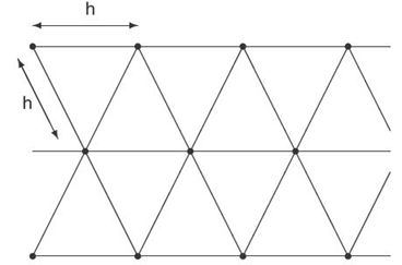
How can we describe this distance in terms of the density ρ_s(x)? When the density is constant, we want to place the servers in such a way that the largest distance r to a server is as small as possible. (Alternatively, if r is fixed, we want to minimize the number of servers for which every point is at a distance ≤ r from one of the servers.) In geometric terms, this means that every point on a plane belongs to a circle of radius r centered on one of the servers—and thus, the whole plane is covered by such circles. Out of all such coverings, we want to find the covering with the smallest possible number of servers.

It is known that the smallest such number is provided by an equilateral triangle grid, that is, a grid formed by equilateral triangles; see, for example, References 7 and 8.

Let us assume that we have already selected the server density functionρ_s(x). Within a small region of area A, we have A·ρ_s(x) servers. Thus, if we, for example, place these servers on a grid with distance h between the two neighboring ones in each direction, we have:

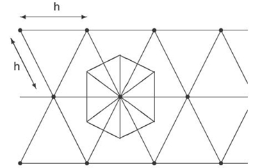
For this placement, the set of all the points that are closest to a given server forms a hexagonal area:

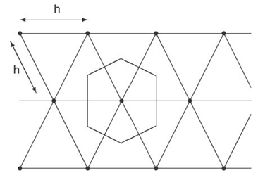
This hexagonal area consists of six equilateral triangles with height h/2:

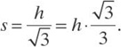
In each triangle, the height h/2 is related to the size s by the formula

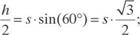
hence,

Thus, the area A_t of each triangle is equal to

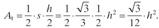
So, the area A_s of the whole set is equal to six times the triangle area:

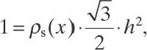
Each point from the region is the closest to one of the points from the server grid, so the region of area A is thus divided into A·ρ_s(x) (practically) disjoint sets of area So, the area of the region is equal to the sum of the areas of these sets:

Dividing both sides of this equality by A, we conclude that

and hence, that

where we denote

The largest distance r to a server is thus equal to

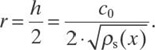
The average distance is proportional to r, since when we rescale the picture, all the distances, including the average distance, increase proportionally. Since the distance r is proportional to (ρ_s(x))^−1/2, the average distance near the location x is thus also proportional to this same value: = const .(ρ_s(x))^−1/2 for some constant.

At each location x, we have ~ρ_r(x) requests. Thus, the total average distance—the value that we would like to minimize—is equal to ρ and is therefore proportional to

So, minimizing the average distance is equivalent to minimizing the value of the above integral.

We want to find the server placement ρ_s(x) that minimizes this integral under the constraint that the total number of server is D, that is, that ∫ρ_s(x)dx = D.

28.2.3    Resulting Constraint Optimization Problem

Thus, we arrive at the following optimization problem:

• We know the density ρ_r(x) and an integer D.
• Under all possible functions ρ_s(x) for which ∫ρ_s(x)dx = D, we must find a function that minimizes the integral ∫(ρ_s(x))^−1/2·ρ_r(x)dx.

28.2.4   Solving the Resulting Constraint Optimization Problem

A standard way to solve a constraint optimization problem of optimizing a function f(X) under the constraint g(X) = 0 is to use the Lagrange multiplier method, that is, to apply unconstrained optimization to an auxiliary function f(X) + λ·g(X), where the parameter λ (called Lagrange multiplier) is selected in such a way so as to satisfy the constraint g(X) = 0.

With respect to our constraint optimization problem, this means that we need to select a density ρ_s(x) that optimizes the following auxiliary expression:

Having an unknown function ρ_s(x) means, in effect, that we have infinitely many unknown values ρ(x) corresponding to different locations, x. Optimum is attained when the derivative with respect to each variable is equal to 0. Differentiating the above expression with respect to each variable ρ_s(x), and equating the result to 0, we get the equation

hence ρ_s(x) = c · (ρ_r(x))^2/3 for some constant c.

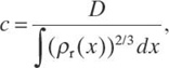
The constant c can be determined from the constraint ∫ρ_s(x) dx = D; that is,

Thus,

and we arrive at the following solution.

28.2.5   Solution to the Problem

Once we know the request density ρ_r(x) and the total number of servers D that we can afford, the optimal server density ρ_s(x) is equal to

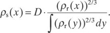
28.2.6   Discussion

In line with common sense, the optimal server density increases when the request density increases, that is,

• in locations that generate more requests, we place more servers, and
• in locations that generate fewer requests, we place fewer servers.

However, when the request density decreases, the server density decreases slower because, otherwise, if we took the server density simply proportional to the request density, the delays in areas with few users would have been huge.

It is worth mentioning that similar conclusions come from the analysis of a different—security-related—optimization problem in which, instead of placing servers, we need to place sensors; see References 8.

28.3   SERVER PLACEMENT IN CLOUD COMPUTING: TOWARD A MORE REALISTIC MODEL

28.3.1   First Idea

In the above first approximation, we took into account only the time that it takes to move the data to the user. This would be all if the database was not changing. In real life, databases need to be periodically updated. Updating also takes time. Thus, when we find the optimal placement of servers, we need to take into account not only expenses on moving the data to the users but also the expenses of updating the information.

How do we estimate these expenses? In a small area, where the user distribution is approximately uniform, the servers are also uniformly distributed; that is, they form a grid with distance h = 2r between the two neighboring servers [7, 8]. Within a unit area, there are ~1/r² servers, and reaching each of them from one of its neighbors requires time proportional to the distance ~r. The overall effort of updating all the servers can be obtained by multiplying the number of servers by an effort needed to update each server and is thus proportional to 1/r²·r ~ 1/r. We already know that r ~ (ρ_s(x))^−1/2; thus, the cost of updating all the servers in the vicinity of a location x is proportional to (ρ_s(x))^1/2. The overall update cost can thus be obtained by integrating this value over the whole area. Thus, we arrive at the following problem.

28.3.2   Resulting Optimization Problem

• We know the density ρ_r(x), an integer D, and a constant C that is determined by the relative frequency of updates in comparison with frequency of normal use of the database.
• Under all possible functions ρ_s(x) for which ∫ρ_s(x) dx = D, we must find a function that minimizes the expression

28.3.3   Solving the Problem

To solve the new optimization problem, we can similarly form the Lagrange multiplier expression

differentiate it with respect to each unknown ρ_s(x), and equate the resulting derivative to 0. As a result, we get an equation,

This is a cubic equation in terms of (ρ_s(x)) ^−1/2, so while it is easy to solve numerically, there is no simple analytical expression as in the first approximation case.

The resulting solution ρ_s(x) depends on the choice of the Lagrange multiplier λ; that is, in effect, we have ρ_s(x) = ρ_s(x, λ). The value λ can be determined from the condition that ∫ρ_s(x, λ) dx = D.

28.3.4   Second Idea

The second idea is that, usually, a service provides a time guarantee, so we should require that, no matter where a user is located, the time for this user to get the desired information from the database should not exceed a certain value. In our model, this means that a distance r from the user to the nearest server should not exceed a certain given value r₀. Since r ~ (ρ_s(x))^−1/2, this means, in turn, that the server density should not decrease below a certain threshold, ρ₀.

This is an additional constraint that we impose on ρ_s(x). In the first approximation model, it means that instead of the formula ρ_s(x) = c·(ρ_r(x))^2/3, which could potentially lead to server densities below ρ₀, we should have ρ_s(x) = max c·(ρ_r(x)) ^2/3, ρ₀).

The parameter c can be determined from the constraint

Since the integral is an increasing function of c, we can easily find the solution c of this equation by bisection (see, e.g., References 9).

28.3.5   Combining Both Ideas

If we take both ideas into account, then we need to consider only those roots of the above cubic equation that are larger than or equal to ρ₀; if all the roots are <ρ₀, we take ρs(x) = ρ.

The resulting solution ρ_s(x) depends on the choice of the Lagrange multiplier λ; that is, in effect, we have ρ_s(x) = ρ_s(x, λ). The corresponding value λ can also be similarly determined from the equation ∫ρ_s(x, λ)dx = D.

28.4   PREDICTING CLOUD GROWTH: FORMULATION OF THE PROBLEM AND OUR APPROACH TO SOLVING THIS PROBLEM

28.4.1   Why It is Important to Predict the Cloud Growth

In the previous sections, when selecting the optimal placement of servers, we assumed that we know the distribution of users'requests; that is, we know the density ρ_r(x). In principle, the information about the users'locations and requests can be determined by recording the users'requests to the cloud.

However, cloud computing is a growing enterprise, so when we plan to select the server's location, we need to take into account not only the current users'locations and requests but also their future requests and locations. In other words, we need to be able to predict the growth of the cloud—both of the cloud in general and of the part corresponding to each specific user location. In other words, we need to predict, for each location x, how the corresponding request density ρ_r(x) changes with time. This density characterizes the size s(t) of the part of the cloud that serves the population located around x.

In the following text, we will refer to this value s(t) as simply “cloud size,” but what we will mean is the size of the part of the cloud that serves a certain geographic location (e.g., the United States as whole or the Southwest part of the United States). Similarly, for brevity, we will refer to the increase in s(t) as simply “cloud growth.”

28.4.2   How We Can Predict the Cloud Growth

To predict the cloud growth, we can use the observed cloud size s(t) at different past moments of time t. Based on these observed values, we need to predict how the rate ds/dt with which the size changes depends on the actual size, that is, to come up with a dependence ds/dt = f(s) for an appropriate function f(s), and then use the resulting differential equation to predict the cloud size at future moments of time.

28.4.3   Why This Prediction is Difficult: The Problem of Uncertainty

The use of differential equations to predict the future behavior of a system is a usual thing in physics: This is how Newton's equations work; this is how many other physical equations work. However, in physics, we usually have a good understanding of the underlying processes, an understanding that allows us to write down reasonable differential equations—so that often, all that remains to be done is to find the parameters of these equations based on the observations. In contrast, we do not have a good understanding of factors leading to the cloud growth. Because of this uncertainty, we do not have a good understanding of which functions should be used to predict the cloud growth.

28.4.4   Main Idea of Our Solution: Uncertainty Itself Can Help

The proposed solution to this problem is based on the very uncertainty that is the source of the problem.

Specifically, we take into account that the numerical value of each quantity—in particular, the cloud size—depends on the selection of the measuring unit. If, to measure the cloud size, we select a unit that is λ times smaller, then instead of the original numerical value s, we get a new numerical value, s′ = λ·s. The choice of a measuring unit is rather arbitrary. We do not have any information that would enable us to select one measuring unit and not the other one. Thus, it makes sense to require that the dependence f(s) look the same no matter what measuring unit we choose.

28.5   PREDICTING CLOUD GROWTH: FIRST APPROXIMATION

28.5.1   How to Formalize This Idea: First Approximation

How can we formalize the above requirement? The fact that the dependence has the same form irrespective of the measuring unit means that when we use the new units, the growth rate takes the form f(s′) = f(λ·s). Thus, in the new units, we get a differential equation ds′/dt = f(s′). Substituting s′ = λ·s into both sides of this equation, we get λ·ds/dt = f(λ·s). We know that ds/dt = f(s), so we get f(λ·s) = λ·f(s).

28.5.2   Solution to the Corresponding Problem

From the above equation, for s = 1, we conclude that f(λ) = λ·const, that is, that f(s) = c·s for some constant c.

As a result, we get a differential equation: ds/dt = f(s) = c·s. If we move all the terms containing the unknown function s to one side of this equation and all the other terms to the other side, we conclude that ds/s = c·dt. Integrating both sides of this equation, we get ln(s) = c·t + A for some integration constant A. Exponentiating both sides, we get a formula, s(t) = a·exp(c·t) (with a = exp(A)), which describes exponential growth.

28.5.3   Limitations of the First Approximation Model

Exponential growth is a good description for a certain growth stage, but in practice, the exponential function grows too fast to be a realistic description on all the growth stages. It is therefore necessary to select more accurate models.

28.6   PREDICTING CLOUD GROWTH: SECOND APPROXIMATION

28.6.1   Second Approximation: Main Idea

While it makes sense to assume that the equations remain the same if we change the measuring unit for cloud size, this does not mean that other related units do not have to change accordingly if we change the cloud size unit. In particular, it is possible that if we change a unit for measuring the cloud size, then to get the same differential equation, we need to select a different unit of time, a unit in which the numerical value of time takes the new form t′ = μ·t for some value μ, which, in general, depends on λ. Thus, in the new units, we have a differential equation, ds′/dt′ = f(s′). Substituting s′ = λ·s and t′ = μ(λ)·t into both sides of this equation, we get λ/μ(λ)·ds/dt = f(λ·s). We know that ds/dt = f(s), so we get f(λ·s) = g(λ)·f(s), where we denoted

28.6.2   Solving the Corresponding Problem

If we first apply the transformation with λ₂ and then with λ₁, we get

On the other hand, if we apply the above formula directly to λ = λ₁·λ₂, we get

By comparing these two formulas, we conclude that g(λ₁·λ₂) = g(λ₁)·g(λ₂). It is well known that every continuous solution to this functional equation has the form g(λ) = λ^q for some real number q;see, for example, References 10. Thus, the equation f(λ·s) = g(λ)·f(s) takes the form f(λ·s) = λ^q·f(s).

From this equation, for s = 1, we conclude that f(λ) = λ^q·const, that is, that f(s) = c·s^q for some constants c and q. As a result, we get a differential equation, ds/dt = f(s) = c·s^q. If we move all the terms containing the unknown function s to one side of this equation and all the other terms to the other side, we conclude that

We have already considered the case q = 1. For q ≠ 1, integrating both sides of this equation, we conclude that s^1−q = c·t + A for some integration constant A. Thus, we get s = C·(t + t₀) ^b for some constants C and b(with b = 1/(q − 1)). In particular, if we start the time with the moment when there was no cloud, when we had s(t) = 0, then this formula takes the simpler form s(t) = C·t^b.

This growth model is known as the power function model; see, for example, References 11‒13.

28.6.3   Discussion

The power function model is a better description of growth than the exponential model, for example, because it contains an additional parameter that enables us to get a better fit with the observed values s(t). However, as mentioned in References 12 and 13, this model is relatively rarely used to describe the growth rate, since it is viewed as a empirical model, a model that lacks theoretical foundations, and is therefore less reliable: We tend to trust more those models that are not only empirically valid, but also follow from some reasonable assumptions.

In the above text, we have just provided a theoretical foundation for the power function model, namely, we have shown that this model naturally follows from the reasonable assumption of unit independence. We therefore hope that with such a theoretical explanation, the empirically successful power function model will be perceived as more reliable—and thus, it will be used more frequently.

28.6.4   Limitations of the Power Function Model

While the power function model provides a reasonable description for the actual growth rate—usually a much more accurate description than the exponential model—this description is still not perfect. For example, in this model, the growth continues indefinitely, while in real life, the growth often slows down and starts asymptotically reaching a certain threshold level.

28.7   PREDICTING CLOUD GROWTH: THIRD APPROXIMATION

28.7.1   Third Approximation: Main Idea

To achieve a more accurate description of the actual growth, we need to have growth models with a larger number of parameters that can be adjusted to observations. A reasonable idea is to consider, instead of a single growth function f(s), a linear space of such functions, that is, to consider functions of the type f(s) = c₁·f₁(s) + c₂·f₂(s) + ⋯ + c_n·f_n(s), where f₁(s), ⋯, f_n(s) are given functions and c₁, ⋯, c_n are parameters that can be adjusted based on the observations.

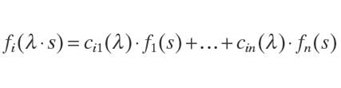
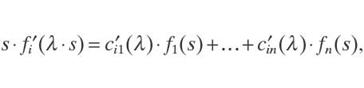
Which functions f_i(s) should be chosen? Our idea is the same as before: Let us use the functions f_i(s) for which the change in the measuring unit does not change the class of the corresponding functions. In other words, if we have a function f(s) from the original class, then, for every λ, the function f(λ·s) also belongs to the same class. Since the functions f(s) are linear combinations of the basic functions f_i(s), it is sufficient to require that this property be satisfied for the functions f_i(s), that is, that we have

for appropriate values c_ij(λ) depending on λ.

28.7.2   Solving the Corresponding Problem

It is reasonable to require that the functions f_i(s) be smooth (differentiable). In this case, for each i, if we select n different values s₁, ⋯, s_n, then for n unknowns c_i1(λ), ⋯, c_in(λ), we get a system of n linear equations:

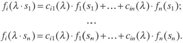
By using Cramer's rule, we can describe the solutions c_ij (λ) of this system of equations as a differentiable function in terms of f_i(λ·s_j) and f_i(s_j). Since the functions f_i are differentiable, we conclude that the functions c_ij(λ) are differentiable as well. Differentiating both sides of the equation

with respect to λ, we get

where g′ denotes the derivative of the function g. In particular, for λ = 1, we get

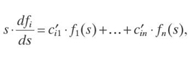
where we denoted . This system of differential equations can be further

simplified if we take into account that ds/s = dS, where . Thus, if we take a new variable S = ln(s) for which s = exp(S) and new unknowns the above equations take a simplified form:

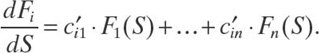
This is a system of linear differential equations with constant coefficients. A general solution of such a system is well known: It is a linear combination of functions of the type exp(a·S), s^k·exp(a·S), exp(a·S)·cos(b·S + φ), and s^k·exp(a·S)·cos(b·S + φ).

To represent these expressions in terms of s, we need to substitute S = ln(s) into the above formulas. Here,

Thus, we conclude that the basic functions f_i(s) have the form s^a, s^a·(1n(s))^k, s^a·cos(b·ln(s) + φ), and s^a·cos(b·ln(s) + φ)·(1n(s)) ^k.

28.7.3   Discussion

Models corresponding to f_i(s) = s^ai have indeed been used to describe the growth; see, for example, References 12 and 13. In particular, if we require that the functions f_i(s) be not only differentiable but also analytical, we then conclude that the only remaining functions are monomials f_i(s) = sⁱ. In particular, if we restrict ourselves to monomials of second order, we thus get growth functions f(s) = c₀ + c₁·s + c₂·s². Such a growth model is known as the Bass model [12‒14]. This model describes both the almost-exponential initial growth stage and the following saturation stage.

Oscillatory terms s^a·cos(b·ln(s) + φ) and s^a·cos(b·ln(s) + φ)·(ln(s))^k can then be used to describe the fact that, in practice, growth is not always persistent; periods of faster growth can be followed by periods of slower growth and vice versa.

In the above description, we assumed that at each moment of time t and for each location x, the state of the part of the cloud that serves requests from this location can be described by a single parameter—its size, s(t). In practice, we may need several related parameters, s⁽¹⁾(t), ⋯, s^(k)(t), to describe the size of the cloud: the number of nodes, the number of users, the amount of data processing, and so on. Similar models can be used to describe the growth of two or more dependent growth parameters:

For example, in the analytical case, the rate of change of each of these parameters is a quadratic function of the current values of these parameters:

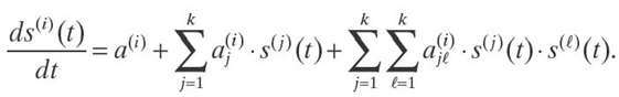
For k = 2, such a model was proposed by Givon et al. [13, 15].

Similar models can be used to describe expenses related to cloud computing; see the Appendix.

28.8   CONCLUSIONS AND FUTURE WORK

28.8.1   Conclusions

This chapter presents the mathematical solutions for two related cloud computing issues: server placement and cloud growth prediction. For each of these two problems, we first list the simplifying assumptions then give the derivation of the corresponding model and the solutions. Then, we relax the assumptions and give the solution to the resulting more realistic models.

28.8.2   Future Work

The server placement problem is very similar to the type of problems faced by Akamai and other companies that do web acceleration via caching; we therefore hope that our solution can be of help in web acceleration as well.

ACKNOWLEDGMENTS

This work was supported in part by the National Center for Border Security and Immigration, by the National Science Foundation grants HRD-0734825 and DUE-0926721, and by Grant 1 T36 GM078000-01 from the National Institutes of Health. The author is thankful to the anonymous referees for useful advice.

Appendix

Description of Expenses Related to Cloud Computing

ANALYSIS OF THE PROBLEM

The chapter [16] analyzes how the price per core C_coredepends on the per-core throughput T_core and on the number of cores N_core.

Some expenses are needed simply to maintain the system, when no computations are performed and T_core = 0. In other words, in general, C_core(0) ≠ 0. It is therefore desirable to describe the additional expenses caused by computations as a function of these computations 'intensity. Thus, we would like to fi nd a function f_sfor which △C_core≈ f(T_core).

MAIN IDEA

Similar to the growth case, we can use the uncertainty to require that the shape of this dependence f(s) does not depend on the choice of a unit for measuring the throughput—provided that we correspondingly change the unit for measuring expenses.

RESULTING FORMULA

As a result, we get a power law, △C_core≈c_T^.(T_core)^b; in other words, C_core ≈ a + c_T^.(T_core)^b, where we denoted .

DISCUSSION

Empirically, the above formula turned out to be the best approximation for the observed expenses [16]. Our analysis provides a theoretical justification for this empirical success.

DEPENDENCE ON THE NUMBER OF CORES IN A MULTICORE COMPUTER

A similar formula, C_core ≈ a + c_N^.(N_core)^d can be derived for describing how the cost per core depends on the number of cores N_core. This dependence is also empirically the best [16]. Thus, our uncertainty-based analysis provides a justification for this empirical dependence as well.

REFERENCES

[1] A. Gates, V. Kreinovich, L. Longpré, P. Pinheiro da Silva, and G.R. Keller, “Towards secure cyberinfrastructure for sharing border information,” in Proceedings of the Lineae Terrarum: International Border Conference, pp. 27‒30, El Paso, Las Cruces, and Cd. Juarez, March 2006.

[2] G.R. Keller, T.G. Hildenbrand, R. Kucks, M. Webring, A. Briesacher, K. Rujawitz, A.M. Hittleman, D.J. Roman, D. Winester, R. Aldouri, J. Seeley, J. Rasillo, T. Torres, W.J. Hinze, A. Gates, V. Kreinovich, and L. Salayandia, “A community effort to construct a gravity database for the United States and an associated Web portal,” in Geoinformatics: Data to Knowledge(A.K. Sinha, ed.), pp. 21‒34. Boulder, CO: Geological Society of America Publications, 2006.

[3] L. Longpré and V. Kreinovich, “How to efficiently process uncertainty within a cyber-infrastructure without sacrificing privacy and confidentiality,” in Computational Intelligence in Information Assurance and Security(N. Nedjah, A. Abraham, and L. de Macedo Mourelle, eds), pp. 155‒173. Berlin: Springer-Verlag, 2007.

[4] P. Pinheiro da Silva, A. Velasco, M. Ceberio, C. Servin, M.G. Averill, N. Del Rio, L. Longpr é, and V. Kreinovich, “Propagation and provenance of probabilistic and interval uncertainty in cyberinfrastructure-related data processing and data fusion,” in Proceedings of the International Workshop on Reliable Engineering Computing REC'08(R.L. Muhanna and R.L. Mullen, eds.), pp. 199‒234, Savannah, GA, February 20‒22, 2008.

[5] A.K. Sinha, ed., Geoinformatics: Data to Knowledge. Boulder, CO: Geological Society of America Publications, 2006.

[6] O. Lerma, E. Gutierrez, C. Kiekintveld, and V. Kreinovich, “Towards optimal knowledge processing: From centralization through cyberinsfrastructure to cloud computing,”International Journal of Innovative Management, Information & Production (IJIMIP), 2(2): 67‒72, 2011.

[7] R. Kershner, “The number of circles covering a set,”American Journal of Mathematics, 61(3): 665‒671, 1939.

[8] C. Kiekintveld and O. Lerma, “Towards optimal placement of bio-weapon detectors,” in Proceedings of the 30th Annual Conference of the North American Fuzzy Information Processing Society NAFIPS'2011, pp. 18‒20, El Paso, Texas, March 2011.

[9] T.H. Cormen, C.E. Leiserson, R.L. Rivest, and C. Stein, Introduction to Algorithms. Cambridge, MA: MIT Press, 2009.

[10] J. Aczel, Lectures on Functional Differential Equations and their Applications. New York: Dover, 2006.

[11] G. Kenny, “Estimating defects in commerical software during operational use,” IEEE Transactions on Reliability, 42(1): 107‒115, 1993.

[12] H. Pham, Handbook of Engineering Statistics. London: Springer-Verlag, 2006.

[13] G. Zhao, J. Liu, Y. Tang, W. Sun, F. Zhang, X. Ye, and N. Tang, “Cloud computing: A statistics aspect of users,” in CloudComp 2009, Springer Lecture Notes in Computer Science (M.G. Jattun, G. Zhao, and C. Rong, eds), Vol. 5931, pp. 347‒358. Berlin: Springer-Verlag, 2009.

[14] F.M. Bass, “A new product growth for model consumer durables,”Management Science, 50 (Suppl.12): 1825‒1832, 2004.

[15] M. Givon, V. Mahajan, and E. Muller, “Software piracy: Estimation of lost sales and the impact of software diffusion,” Journal of Marketing, 59(1): 29‒37, 1995.

[16] H. Li and D. Scheibli, “On cost modeling for hosetd enterprise applications,” in CloudComp 2009, Lecture Notes of the Institute of Computer Sciences, Social-Informatics, and Telecommunications Engineering (D.R. Avresky, ed.), Vol.34, pp. 261‒269. Heidelberg: Springer-Verlag, 2010.