
CHAPTER 7
MULTI VARIATE TECHNIQUES WITH TEXT
Data is collected by taking measurements. These are often unpredictable, for one of two reasons. First, there is measurement error, and, second, the objects measured can be ran– domly selected as discussed in section 6.2. Random variables can model either type of unpredictability.
Text mining often analyzes multiple texts. For example, there are 68 Edgar Allan Poe short stories, all of which are of interest to a literary critic. A more extreme example is a researcher analyzing the EnronSent corpus. This has about a 100 megabytes of text, which translates into a vast number of emails.
Hence, a text miner often has many variables to analyze simultaneously. There are a number of techniques for this situation, which are collectively called multivariate statistics. This chapter introduces one of these, principal components analysis (PCA).
This chapter focuses on applications, and some of the key ideas of PCA are introduced. The goal is not to explain all the details, but to give some idea about how it works, and how to apply it to texts. Specifically, 68 Poe short stories are analyzed. These are from a five volume collected work that is in the public domain and is available online ([96], [97], [98], [99] and [100]).
These 68 stories are “The Unparalleled Adventures of One Hans Pfaall," “The Gold Bug," “Four Beasts in One," “The Murders in the Rue Morgue," “The Mystery of Marie Rogêt," “The Balloon Hoax," “MS. Found in a Bottle," “The Oval Portrait," “The Purloined Let– ter," “The Thousand-and-Second Tale of Scheherezade," “A Descent into the MaelstrÖm," “Von Kempelen and His Discovery," “Mesmeric Revelation," “The Facts in the Case of M. Valdemar," “The Black Cat," “The Fall of the House of Usher," “Silence – a Fable," “The Masque of the Red Death," “The Cask of Amontillado," “The Imp of the Perverse," “The Island of the Fay," “The Assignation," “The Pit and the Pendulum," “The Premature Burial," “The Domain of Arnheim," “Landor’s Cottage," “William Wilson," “The Tell-Tale Heart," “Berenice," “Eleonora," “Ligeia," “Morella," “A Tale of the Ragged Mountains," “The Spectacles," “King Pest," “Three Sundays in a Week," “The Devil in the Belfry," “Li– onizing," “X-ing a Paragrab," “Metzengerstein," “The System of Doctor Tarr and Professor Fether," “How to Write a Blackwood Article," “A Predicament," “Mystification," “Did– dling," “The Angel of the Odd," “Mellonia Tauta," “The Duc de l’Omlette," “The Oblong Box," “Loss of Breath," “The Man That Was Used Up," “The Business Man," “The Land– scape Garden," “Maelzel’s Chess-Player," “The Power of Words," “The Colloquy of Monas and Una," “The Conversation of Eiros and Charmion," “Shadow –A Parable," “Philosophy of Furniture," “A Tale of Jerusalem," “The Sphinx," “Hop Frog," “The Man of the Crowd," “Never Bet the Devil Your Head," “Thou Art the Man," “Why the Little Frenchman Wears His Hand in a Sling," “Bon-Bon," and “Some Words with a Mummy." Although “The Lit– erary Life of Thingum Bob, Esq." is listed in the contents of Volume 4, it is not in any of the five volumes.
These 68 stories are used as is except for the following. First, all the footnotes are removed except for the story “The Unparalleled Adventures of One Hans Pfaall," where Poe discusses other moon tales. Second, the XML tags <TITLE> and </TITLE> are placed around each story title. Third, each story has a notice marking the end of it, and these are removed.
The next section starts with some simpler statistical ideas that are needed for PCA. Fortunately, the amount of mathematics and statistics needed is not as much as one might fear.
Section 4.4 introduces the mean and variance of a random variable as well as the sample mean and sample standard deviation of a data set. It is pointed out that these are easiest to interpret if the data has a bell shape (that is, the population is approximately a normal distribution). For an example, see figure 4.4.
Since language is generative, any group of texts can be considered a sample from a large population of potential texts. For example, Poe wrote about 68 short stories in his lifetime, but if he lived longer (he died at age 40) he would have written more. Undoubtably, he probably had many other ideas for stories, which he might have written given different circumstances such as if he were more financially successful during his life. Hence, we focus on sample statistics.
Suppose a data set has the values x1, x2,...xn where n represents the sample size. The sample mean is given in equation 7.1.
(7.1)![]()
For bell-shaped data, the sample mean is a typical value of this data set. But the shape of the data set is an important consideration; for example, if the histogram of a data set is bimodal (has two peaks), the mean can be atypical.
Equation 7.2 for the sample variance is more complex. Note that the sum is divided by n – 1, not n, so this is not quite a mean of the squared terms in the sum. However, if n is large, n – 1 is close to n.
(7.2)![]()
The sample variance is a measure of the variability of the data. Thinking in terms of histograms, generally the wider the histogram, the more variable the data, and the least variable data set has all its values the same. In fact, no variability implies that s2x equals zero. Conversely, if s2x is zero, then every data value is the same. See problem 7.1 for an argument why this is true.
Note that s2x measures the variability about ![]() . Equation 7.2 implies this is true because the only way xi, can contribute to s2x is if it differs from
. Equation 7.2 implies this is true because the only way xi, can contribute to s2x is if it differs from ![]() . Note that if xi is less than
. Note that if xi is less than ![]() , this difference is negative, but squaring it makes a positive contribution. Other functions can be used to make all these differences nonnegative, for example, the absolute value. However, squaring has theoretical advantages; for example, it is easy to differentiate, which makes it easier to optimize sums of squares than, say, sums of absolute values.
, this difference is negative, but squaring it makes a positive contribution. Other functions can be used to make all these differences nonnegative, for example, the absolute value. However, squaring has theoretical advantages; for example, it is easy to differentiate, which makes it easier to optimize sums of squares than, say, sums of absolute values.
For data analysis, the square root of the variance, sx, is used, which is called the sample standard deviation. Note that ![]() and sx have the same units as the data set. For example, if the data consists of sentence lengths in terms of word counts, then
and sx have the same units as the data set. For example, if the data consists of sentence lengths in terms of word counts, then ![]() and sx are word counts. If the data were sentence lengths in letter counts, then
and sx are word counts. If the data were sentence lengths in letter counts, then ![]() and sx are letter counts. Note that variance is in squared units. For example, the variance of a data set of times measured in seconds (s) is a number with units s2 or seconds squared. The next section describes an important application of the sample mean and sample standard deviation.
and sx are letter counts. Note that variance is in squared units. For example, the variance of a data set of times measured in seconds (s) is a number with units s2 or seconds squared. The next section describes an important application of the sample mean and sample standard deviation.
7.2.1 z-Scores Applied to Poe
A z-score is a way to compute how a data value compares to a data set. It converts this value to a number, which is dimensionless, that is, there are no units of measurement left. Specifically, it measures the number of standard deviations a value is from the mean of its data set.
The formula for the z-score of x is given in equation 7.3. Since both the numerator and denominator have the same units, these cancel out.
(7.3)![]()
As an example, we compute z-scores for word lengths of the 68 Poe short stories. In programming, once a task works for one particular example, it is often straightforward to apply it to numerous examples.
For computing ![]() , only a running count and sum are needed. Equation 7.2 for the sample standard deviation, however, requires knowing
, only a running count and sum are needed. Equation 7.2 for the sample standard deviation, however, requires knowing ![]() first, so a program using it needs to go through the text twice. However, there is an equivalent form of this equation that only requires a running sum of the squares of the values. This is given in equation 7.4.
first, so a program using it needs to go through the text twice. However, there is an equivalent form of this equation that only requires a running sum of the squares of the values. This is given in equation 7.4.
(7.4)![]()
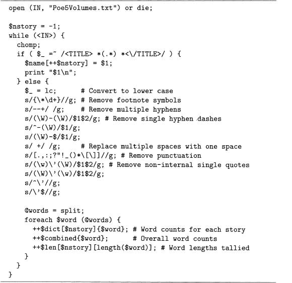
The words are identified by code sample 7.1, which removes the punctuation. Note that any apostrophes that start or end the word are removed. For instance, Excellencies ‘pleasure loses its apostrophe, which is not the case with friend’s equanimity. However, the challenge of correctly identifying possessive nouns ending in -s is greater than the payoff, so it is not done. Compare this with program 5.2, which analyzes four Poe stories.
Code Sample 7.1 This code removes punctuation, counts words, and computes word lengths for each Poe story.
Code sample 7.2 uses the array of arrays len of code sample 7.1 to compute the mean, variance, and standard deviation of the word lengths for the 68 Poe short stories. Note that the first for statement ioops through all the stories, and the second one loops through all the words in each story. As claimed above, by using equation 7.4, only one pass through all the words is needed.
Code Sample 7.2 Code to compute the sample mean, sample variance, and sample standard deviation for each Poe story. To run, append this to code sample 7.1.
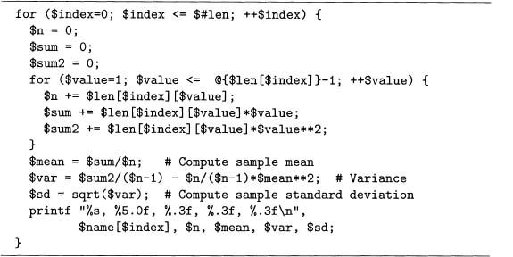
By adding code sample 7.2 to the end of code sample 7.1, the result produces 68 lines of output. Each has the following form, where the first number is the length of the story in words, the second is the sample mean, the third is the sample variance, and the fourth is the sample standard deviation.
THE GOLD-BUG, 13615, 4.305, 6.135, 2.477
With these means and standard deviations, it is possible to compute z-scores of any word length for each story. Let us do this for a four-letter word. The z-score of 4 for “The Gold-Bug" is given in equation 7.5.
(7.5)![]()
This means that for “The Gold-Bug," a word length of 4 is 0.123 standard deviations below the mean. This varies from story to story. The extreme z-scores are – 0.0100 for “Why the Little Frenchman Wears His Hand in a Sling" and – 0.3225 for “Metzengerstein." So four-letter words are all slightly below average for all the stories.
Although z-scores are computable for any data set, it is easier to interpret for approxi–mately bell-shaped data. However, word lengths are not symmetric around the mean: there are fewer values less than the mean than are greater than it. For example, see output 3.4 for “The Tale-Tell Heart." This data shape is called right skewed. Nonetheless, there is only one peak; that is, it is unimodal. In addition, the longest word has 14 letters, so there are no extremely long words in this story. For such data, z-scores can still be useful.
Although z-scores are valuable themselves, they are also useful in computing correlations. This is the topic of the next section.
7.2.2 Word Correlations among Poe’s Short Stories
For comparing two variables, units are a problem. For example, how should a physicist compare masses and times? One solution is to convert both variables to z-scores, and then compare these.
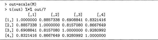
Another solution is the sample correlation coefficient. Equation 7.6 shows how to compute this, and notice that it is almost the mean of the product of the z-scores of each data value.
(7.6)![]()
Correlations are used in a variety of statistical techniques, including PCA. It can be proved that the correlation r must satisfy equation 7.7.
(7.7)![]()
Both r = 1 and r = –1 constrain the data to lie on a line when plotted. That is, both require that one variable is a linear function of the other. When r = 1, this has a positive slope, and r = –1 implies a negative slope. When r = 0, there is no linear relationship between the two variables. However, for all values of r, nonlinear relationships are possible.
For the first example, we analyze the frequencies of some common function words ir each of the 68 Poe stories. It is likely that these counts are roughly proportional to the size of each story. If this is true, then these counts are positively correlated.
One way to detect a trend in the data is to plot two variables at a time in a scatter plot which we do in R. Because this requires reading the data into R, it makes sense to have ii compute the correlations, too, instead of programming Perl to do so. Although equation 7.6 is not that complicated, it is still easier to let a statistical software package do the work.
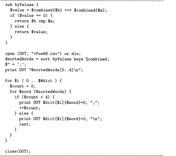
Code sample 7.3 computes a term-document matrix when it is combined with code sample 7.1. The open statement stores this matrix in the comma-separated file, Poe68. csv which is sorted by the word frequencies of all 68 stories combined. Since this is a large file with 68 columns and over 20,000 rows, we consider just the top five words: the, of, and, a and to. For how this is done in code sample 7.3, see problem 7.2.
Code Sample 7.3 Creating a transposed term-document matrix for the 68 Poe stories and 5 most frequent words. This uses @dict from code sample 7.1.
Reading Poe68. csv into R is done with read. csvO. Remember that the greater than character is the command prompt for this package. The first argument is the filename, an note that a double backslash for the file location is needed. The second argument, header=T means that the first row contains the variable names.
The values are stored in data, which is called a data frame. The name data refers tc the entire data set, and each variable within it is accessible by appending a dollar sign to this name, then adding the column name. For example, the counts for the word the are ir data$the.
> data = read.csv("C:\Poe68.csv", header=T)
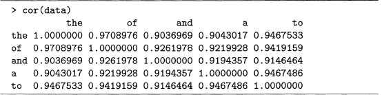
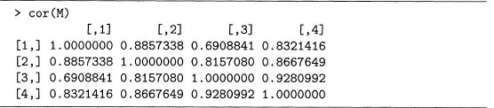
The cor () function computes the correlations as shown in output 7.1. These are or–; ganized in a five by five table. Each entry on the main diagonal is 1, which must be true because any variable equals itself, which is a linear function with positive slope.
This matrix of correlations is symmetric about the main diagonal. For example, the correlation between of and the is the same as the correlation between the and of. So this matrix can be summarized by a triangular table of values. However, there are mathematical reasons to use the full matrix, which are discussed in section 7.3.
Looking at the off-diagonal values, all the correlations are above 0.90, which are large Using the function pairs (), the positive trends are easily seen in figure 7.1, even though each individual plot is small.
Figure 7.1 Plotting pairs of word counts for the 68 Poe short stories.
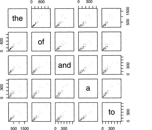
> pairs(data, pch=’.’)
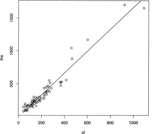
In figure 7.2, the counts of of and the are compared in one plot. In addition, the optimal prediction line is drawn. Output 7.2 gives the R commands to create both the plot and this line, which is called the regression line.
Figure 7.2 Plots of the word counts for the versus of using the 68 Poe short stories.
Output 7.1 Example of computing correlations in R.
The function attach() makes the variables in data accessible by just using the column name. For example, data$the can be replaced with the. Hence plot (of ,the) is a plot of the word counts of of and the for each of the 68 Poe stories.
The function lm() fits a linear model of the variable before the tilde as a function of all of them after it. So in output 7.2, the counts of the are modeled as a linear function of the of counts. The result is shown in output 7.3, which implies equation 7.8. Problem 7.3 shows how to get more information about the results of lm ().
(7.8)![]()
Output 7.2 Making a plot with the regression line added for the word counts of the versus of.
> attach(data) |
> plot(of,the) |
> lmofthe = lm(the ~ of) |
> lines(of, fitted(lmofthe)) |
The function fitted() returns the predicted values given by equation 7.8. Output 7.2 uses these to add the regression line using the command lines 0, as shown below.
> lines(of, fitted(lmofthe))
The above discussion introduces the correlation. However, this computation is closely related to the cosine similarity measure introduced in section 5.4. The connection between these two techniques is explained in the next section.
7.2.3 Correlations and Cosines
This link between cosines and correlations is easy to show mathematically. Suppose the two variables X and Y have means equal to zero, that is, ![]() =
= ![]() = 0. Then equation 7.9 holds true.
= 0. Then equation 7.9 holds true.
(7.9)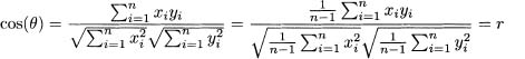
Output 7.3 Fitting a linear function of the counts of the as a function of the counts of of for each Poe story. Output 7.2 computes imofthe.
> imofthe | |
Call: | |
lm(formula = the ~ of) | |
Coefficients: | |
(Intercept) | of |
–;0.03825 | 1.66715 |
Of course, data rarely has mean zero. However, if xi are measurements of any variable, then it is easy to show that xi – ![]() has mean zero. Note that this expression appears in the numerator of both the z-score (equation 7.3) and the correlation (equation 7.6).
has mean zero. Note that this expression appears in the numerator of both the z-score (equation 7.3) and the correlation (equation 7.6).
Section 5.5.1 shows how to compute the cosines for the term-document matrix given in output 5.3. If this matrix is modified so that each column has mean zero, then the cosines for the modified matrix is exactly the same as the correlation matrix of the original, which is demonstrated in output 7.4. This uses the method shown in output 5.12.
Output 7.4 Example of computing cosines using matrix multiplication.
Output 7.5 The correlations of the columns of the term-document matrix M.
Hence it is no accident that any correlation is between –1 and 1 because it is equivalent to a cosine, which must be between –1 and 1. Although the data set in output 5.7 does not have zero mean, the cosine similarities and the correlations in output 7.5 are similar. In fact, the ranking of the six pairs of stories from most to least similar is the same for both.
As noted earlier, the correlation matrix is redundant because the upper right corner is a mirror image of the lower left corner. This means that the ith row and jth column entry is equal to the jth row and ith column. Symbolically, we denote the entries by subscripts, so this means Rij= RjiOr written in terms of matrices, equation 7.10 holds.
(7.10)![]()
Finally, correlations are not the only way to compute how two variables relate. The next section defines the covariance matrix, which is closely related to the correlation matrix.
7.2.4 Correlations and Covariances
The correlation between two variables is convenient because it is a pure number without the units of measurement of the data. However, sometimes it is useful to retain the original units, and there is a statistic corresponding to the correlation that does exactly this. It is called the covariance.
The formula for the covariance between two variables is given by equation 7.11. There are two ways to write this. First, Cov(X, Y), and, second,xy 8a Note that sxx is just the variance of X because when Y = X, sxx is the same as s2x in equation 7.2.
(7.11)![]()
Note that the units of sxy are just the product of the units of X and Y, which can be hard to interpret. For example, if X is in feet, and Y is in dollars, then sxy is in foot-dollars.
There is a close relationship between correlations and covariances, which is shown in equation 7.12. Comparing this to equations 7.11 and 7.6 shows that the right-hand side is indeed the correlation. Note that the inverse of n – 1 in front of sxy, sxand sy, all cancel out, like it does in equation 7.9.
(7.12)![]()
Output 7.5 shows that cor () produces a correlation matrix in R. The function coy () similarly produces a covariance matrix, as shown in output 7.6 for the same matrix M used above.
Output 7.6 The covariance matrix of the term-document matrix M.
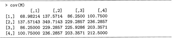
Finally, if the standard deviations of each column of M are computed, then dividing each row and column by its corresponding standard deviation produces the correlation matrix. That is, cor (M) is just a rescaled version of coy (M). See problem 7.4 for more details.
Note that the covariance matrix is also symmetric about its main diagonal. Although both the correlation and the covariance matrices can be summarized with fewer numbers, the next section shows why the square matrix form is useful, which requires some basic ideas from linear algebra.
The last section notes that the correlation matrix for a set of variables is both square (the number of rows equals the number of columns) and symmetric about the main diagonal (the upper right corner is the mirror reflection of the lower left corner). It turns out that such matrices have special properties.
The study of matrices is the focus of linear algebra. It turns out that a fruitful way to understand a matrix, M, is to study how a vector x changes when multiplied by M to get Mx.
Square matrices have at least one nonzero vector that satisfies equation 7.13, where λ is a number. Such vectors are called eigenvectors, and the number λ is called the associated eigenvalue. For these vectors, matrix multiplication is equivalent to multiplication by a number.
(7.13)![]()
It can be proved that n by n correlation and covariance matrices have n real, orthogonal eigenvectors with n real eigenvalues. For example, see theorems 3.8 and 3.10 of Matrix AnalysisforStatistics by Schott [108]. However, instead of theory, the next section discusses the concrete case of the 2 by 2 correlation matrix, which illustrates the ideas needed later in this chapter.
7.3.1 2 by 2 Correlation Matrices
For two variables, the correlation matrix is 2 by 2, and its general form is given in equation 7.14. Note that R is symmetric, that is, RT = R, which is true for any correlation matrix. Our goal is to find the eigenvectors with their respective eigenvalues.
(7.14)![]()
In general, an n by n correlation matrix has n eigenvectors, so R has 2. Call these e1 and e2. By definition, there must be two numbers λ1 and λ2 that satisfy equation 7.15.
(7.15)![]()
Define the matrix E such that its first column is e1, and its second is e2 (E for Eigenvec– tors). Note that RE produces a matrix where the first column is Re1 and its second is Re2. However, these products are known by equation 7.15. Hence, equation 7.17 holds because postmultiplying by a diagonal matrix rescales the columns of the preceding matrix (see output 5.6 for another example of this). Let V be this diagonal matrix (V for eigen Values).
(7.16)![]()
(7.17)![]()
Using the notation of the preceding paragraph, we can rewrite equation 7.17 as equation 7.18. Note that E is not unique. If equation 7.15, is multiplied by any constant, then the result is still true. Hence, e1 can be multiplied by any nonzero constant and remains an eigenvector. One way to remove this ambiguity is to require all the eigenvectors to have length 1, which we assume from now on.
(7.18)![]()
With eigenvectors of unit length, the cosine of the angle between two eigenvectors is the dot product. Note that the transpose of a product of matrices satisfies equation 7.19. For why this is true, see problem 7.5. Since vectors are also matrices, this equation still is true when N is a vector. Using these two facts, it is easy to show that for a correlation matrix, two eigenvectors corresponding to two different nonzero eigenvalues must be orthogonal, that is, the dot product is 0.
(7.19)![]()
To prove this, first note that equation 7.20 requires that RT = R (this is the key property).Then compare equations 7.20 and 7.21. Because both start with the same expression, we conclude that equation 7.22 holds. If λ1 ≠ λ2, then the only way this can happen is when e1Te2 = 0, but this means that the cosine of the angle between these two vectors is zero. Hence these eigenvectors are orthogonal.
(7.20)![]()
(7.21)![]()
(7.22)![]()
In addition, since a vector with unit length implies that the dot product with itself equals 1, then equation 7.23 must hold. Let I be the identity matrix, that is, Iii = 1 and Iij = 0 for i ≠ j. Then equation 7.23 is equivalent to equation 7.24, which holds since matrix multiplication consists of taking the dot product of the rows of the first matrix with the columns of the second matrix. However, the rows of ET are the columns of E, so matrix multiplication in this instance is just taking the dot products of the columns of E, which satisfy equation 7.23. Finally, the second equality in equation 7.24 follows from the first, but proving this requires more mathematics (the concept of inverse matrices), and it is not done here.
(7.23)![]()
(7.24)![]()
A key property of I is that equation 7.25 holds for all vectors x. That is, multiplying vectors by I is like multiplying numbers by 1: the result is identical to the initial value.
(7.25)![]()
With these facts in mind, we can reinterpret equation 7.18 as a way to factor the matrix R. Multiplying this equation on the right by ET (order counts with matrix multiplication: see problem 7.6) and using equation 7.24, we get equation 7.26. Hence, R can be factored into a product of three matrices: the first and last contain its eigenvectors and the middle is a diagonal matrix containing its eigenvalues.
(7.26)![]()
With the theory above in mind, we consider a concrete example. By using the first two columns of the matrix M of output 5.3, we compare the use of male and female pronouns in Poe’s “The Facts in the Case of M. Valdemar" and “The Man of the Crowd." This is done in output 7.7.
Output 7.7 Factoring the correlation matrix of the eight pronouns for the two Poe stories “The Facts in the Case of M. Valdemar" and “The Man of the Crowd."
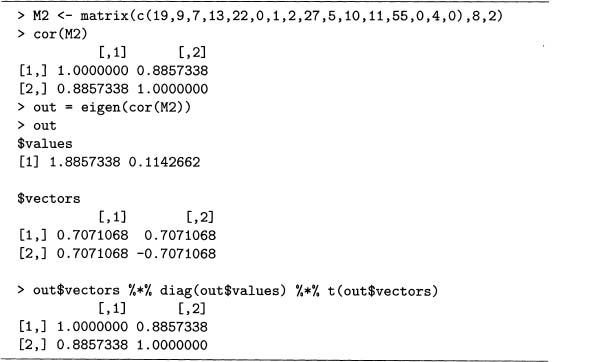
The function eigen() computes the eigenvalues, which are stored in out$values, and the eigenvectors are stored in out$vectors. The last matrix product is the factorization of R = EVET, which matches the output of cor (M2).
Output 7.7 is one particular case of the 2 by 2 correlation matrix, but for this size, the general case is not hard to give, which is done in equation 7.27 through equation 7.30. This reproduces output 7.7 when r = 0.8857338. For example, the eigenvalues are 1 + r and 1 – r, which equal out$values. Note that the second eigenvector in equation 7.28 differs from the second column of out$vectors by a factor of –1. However, this factor does not change the length of this unit vector, so the two answers are interchangeable.
(7.27)![]()
(7.28)![]()
(7.29)![]()
(7.30)![]()
Also note that the eigenvalues 1 + r and 1 — r are always different except when r is zero. Hence, the eigenvalues are always orthogonal when r 0. However, if r = 0, then R = I, and by equation 7.25, all nonzero vectors are eigenvectors (with λ equal to 1). Hence, it is possible to pick two eigenvectors for λ = 1 that are orthogonal, for example, (0,1) and (1,0). Consequently, for all values –1 < r > 1, there are two orthogonal eigenvectors.
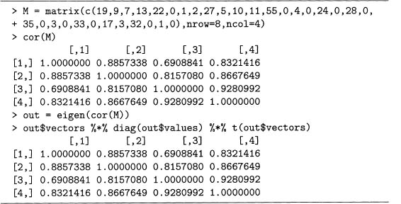
Furthermore, although this section considers the 2 by 2 case, equation 7.24 and the factorization given in equation 7.26 holds for any size correlation matrix. For example, cor (M) in output 5.3 can be factored as well, which is shown in output 7.8.
Output 7.8 Factoring the correlation matrix of the eight pronouns for four Poe stories.
Now we apply the matrix factorization of a correlation matrix R to texts. This is done in the next section with the multivariate statistical technique of principal components analysis.
7.4 PRINCIPAL COMPONENTS ANALYSIS
The ability to reduce a large number of variables to a smaller set is useful. This is especially true when dealing with text since there are numerous linguistic entities to count. Doing this, however, generally loses information. Hence, the goal is to obtain an acceptable trade-off between variable reduction and the loss of information.
Principal components analysis (PCA) reduces variables in a way that as much variability as possible is retained. This approach assumes variability is the useful part of the data, which is plausible in many situations. For example, none of Poe’s 68 short stories has the word hotdog, so each story has 0 instances. Intuitively, this is not as informative as the word counts of death, which varies from 0 to 16.
The approach of PCA is simple. Suppose a data set has the variables x1, x2 xn. Then n new variables, call these c1, c2, ..., cn, are constructed to satisfy the following four conditions. First, each component ci, is a linear function of the original xi variables, so the system of equations 7.31 holds. This is written compactly in matrix notation as follows. Let c be the column vector containing c1, C2... cn let x be the column vector containing x1, x2...xn and let E be the matrix with row i and column j equaling eij. Then equation 7.32 holds.
(7.31)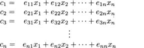
(7.32)![]()
Second, the vector c has unit length. That is, equation 7.33 holds.
(7.33)![]()
Third, each pair of ci and cj (i ≠ j) are uncorrelated. That is, the correlation matrix of c is the identity matrix, I. Fourth, the variances of c1, c2, ..., cn, are ordered from largest to smallest. These four conditions uniquely specify the matrix E, which is given in the next section.
7.4.1 Finding the Principal Components
There are two approaches to PCA. A researcher can work with either the correlation matrix or the covariance matrix. For the former approach, each variable must be converted to its z-scores first. If the latter is used, then the original data values are left alone. Below, both methods are shown, but the focus is on using the correlation matrix, R.
Equation 7.32 puts the PCA coefficients in the matrix E. This might seem like poor notation since E is also used in section 7.3.1 to denote the eigenvector matrix of R. However, it turns out that the columns of R are the PCA coefficients for the z-scores of the data. In addition, the eigenvectors of the covariance matrix are the PCA coefficients for the original data set. For more details on PCA using either the correlation or covariance matrices, see chapter 12 of Rencher’s Methods of Multivariate Analysis [104].
Although R has a function called prcomp () that computes the principal components (PCs), the discussion in the preceding section also allows us to compute these directly using matrix methods. This link between PCA and eigenvectors is applied to a term-document matrices in the next section.
7.4.2 PCA Applied to the 68 Poe Short Stories
Code sample 7.3 gives Perl code to compute the word counts of the five most frequent words in the Poe short stories (namely, the, of, and, a, to). We use this term-document matrix for our first example.
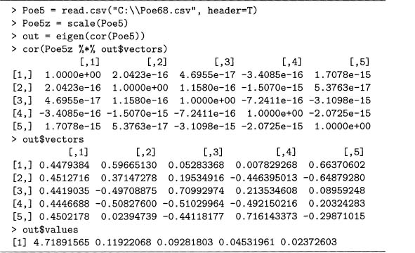
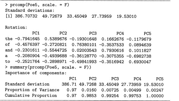
Output 7.9 first reads in the file Poe68. csv by using read. csv (). Then scale () computes the z-scores of the word counts and puts these into the matrix, Poe5z, and out contains both the eigenvectors and eigenvalues of the correlation matrix (note that the correlation matrix of Poe5 is the same as Poe5z since both use z-scores instead of the original data). Taking the product of Poe5z with the eigenvectors produces the PCs. As shown in this output, the correlation matrix of these is the identity matrix, up to round-off error. Finally, out$vectors are both the eigenvectors and the coefficients of the PCs.
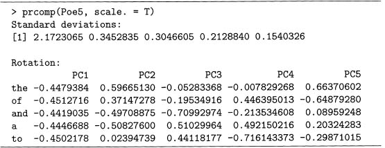
This is also achievable with the function prcomp (), and output 7.10 gives the results. Note that the standard deviations are the square roots of the eigenvalues, and that the PCs are the same as the eigenvectors (up to signs). Setting scale. to true uses the correlation matrix. If it is false, then the covariance matrix is used instead.
Output 7.9 Computing the principal components “by hand.’
Output 7.10 Computing the principal components with the function prcomp (). Compare to output 7.9.
The summary () function shows the importance of each PC in output 7.11. Remember that the first PC is constructed so it gets as much variability as possible, and the second PC gets as much of the rest of the variability as possible, and so forth.
So for these five words, the first PC is roughly proportional to the mean of the counts of the five words since all the weights are approximately equal (and ignoring the negative signs). This PC explains 94.4% of the variability, so the other four PCs are not very important.
Output 7.11 Using suinmary() on the output of prcomp().
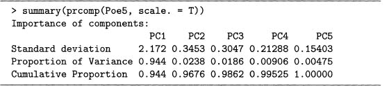
That is, although there are five variables in the data set, these can be summarized by one variable with little loss of variability.
These five words are the most common five words used by Poe in his short stories. In addition, they are all function words, so their counts are positively correlated with the size of the stories. Hence the first PC, which is nearly an average of these counts, captures this relationship.
Finally, note that the PC coefficients differ depending on whether the correlation or covariance matrix is used. This is shown in output 7.12, which computes the PCs using the covariance matrix. Although the coefficients differ, the first PC still explains the vast majority of the variability. So in either case, the five variables can be reduced to one.
Output 7.12 Computing the principal components using the covariance matrix. Compare to output 7.11.
In general, since using the correlation matrix is equivalent to using the z-scores of the data, all the variables have comparable influence in the PCs. Using the covariance matrix, however, implies that the variables that vary most have the most influence. Either case is useful, so it depends on the researcher’s goals on which to use.
The next section briefly looks at another set of word counts for Poe’s stories. This time the variability is more spread out among the PCs.
7.4.3 Another PCA Example with Poe’s Short Stories
In section 5.2.2, the pronouns he, she, him, her, his, hers, himself, and herself are analyzed in four Poe stories. In this section we apply PCA to these using all 68 Poe stories. The counts can be computed by replacing the end of code sample 7.3 with code sample 7.4. The idea is to use the pronouns as keys in the array of hashes, @dict.
Code Sample 7.4 Word counts for the eight pronouns are written to the file Poe68. csv. This requires dict from code sample 7.1.
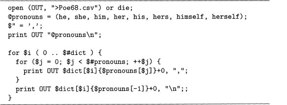
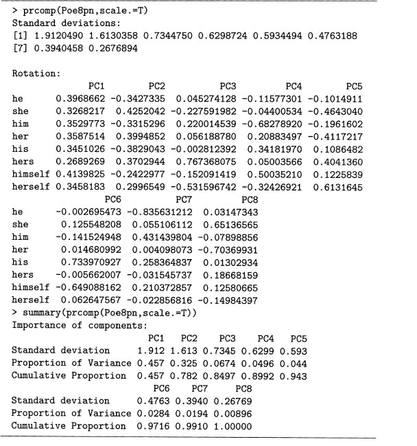
Once the file Poe68. csv is created, read it into R using read. csv (). Then output 7.13 computes the PCA for these eight pronouns.
Again the first PC is approximately proportional to the average of the eight counts since the weights are all roughly the same. Unlike the preceding section, however, the first PC only explains 48% of the variability. Although the second PC also has weights comparable in absolute value, four of the signs are positive, and the other four are negative. Note that the former weights go with the feminine pronouns, and the latter go with the masculine!
Although this PCA uses a bag-of-words language model that ignores all syntactic infor–mation, it distinguishes between male and female pronouns. So using simplified models of language coupled with a computer can discover interesting language structures.
7.4.4 Rotations
Notice outputs 7.10, 7.12, and 7.13 include the word Rotation just before the PCs. This section explains why this is the case.
Rotations only change the orientation but not the shape of any object. For example, spinning a suitcase does not change its shape. Suppose there is a data set with n-variables, then an n-dimensional plot is possible with one dimension for each variable. As with objects, rotating these values changes the orientation but not the shape of the data.
Surprisingly, rotations in any number of dimensions are easy to describe mathematically. Any rotation in n-dimensions is representable by an n-by-n matrix, call it E, that satisfies the two properties given in equations 7.34 and 7.35.
(7.34)![]()
(7.35)![]()
Output 7.13 The PCA of eight pronouns in the 68 Poe short stories.
However, equation 7.34 is the same as equation 7.24. Equation 7.35 it a technical condition that rules out rotations coupled with mirror reflections. Note that det () is the determinant function, which is not discussed in this book, but see section 1.6 of Schott’s Matrix Analysis for Statistics [108] for a definition.
If all the normalized eigenvectors of a correlation matrix are used as the columns of a matrix E, this is a rotation in n-dimensional space. So finding principal components is equivalent to rotating the data to remove all correlations among the variables.
Since rotation does not distort the shape of the data, a PCA preserves all of the informa–tion. Because of this, it is often used to create new variables for other statistical analyses. These new variables have the same informational content as the original ones, and they are uncorrelated.
Information is lost in a PCA only by picking a subset of PCs, but this loss is quantified by the cumulative proportion of variance. This allows the researcher to make an informed decision when reducing the number of variables studied.
The above discussion covers the basics of PCA. The next section gives some examples of text applications in the literature.
7.5.1 A Word on Factor Analysis
The idea of taking a set of variables and defining a smaller group of derived variables is a popular technique. Besides PCA, factor analysis (FA) is often used. Some authors (including myself) prefer PCA to FA, but the latter is well established. Before noting some applications in the literature, this section gives a short explanation on why PCA might be preferred by some over FA.
PCA is based on the fact that it is possible to rotate a data set so that the resulting variables are uncorrelated. There are no assumptions about this data set, and no information is lost by this rotation. Finally the rotation is unique, so no input is needed from the researcher to create the principal components. However, FA is used to reduce the number of variables to a smaller set calledfactors. Moreover, it tries to do this so that the resulting variables seem meaningful to the researcher.
Although FA has similarities to PCA, it does make several assumptions. Suppose this data set has n variables. Then FA assumes that these are a linear function of k factors (k < n), which is a new set of variables. In practice, k factors never fully determine n variables, so assumptions must be made about this discrepancy. FA assumes that these differences are due to random error. Finally, any solution of an FA is not unique: any rotation of the factors also produces a solution. This allows the researcher to search for a rotation that produces factors that are deemed interpretable.
The above discussion reveals two contrasts between these two methods. First, PCA preserves information, but if FA is mistakenly used, then information is lost since it is classified as random error. Second, PCA produces a unique solution, but FA allows the researcher to make choices, which allows the possibility of poor choices.
Since natural languages are immensely complex, the ability of FA to allow researcher bias might give one pause. However, people are experts at language, so perhaps human insight is a valuable input for FA. There is much statistical literature on both of these techniques. For an introduction to PCA and FA, see chapters 12 and 13 of Rencher’s Methods of Multivariate Analysis [104], which includes a comparison of these two methods. For an example of computing an FA in R, see problem 7.8.
The next section notes some applications of PCA and FA to language data sets in the literature. After reading this chapter, these references are understandable.
7.6 APPLICATIONS AND REFERENCES
We start with three non-technical articles. Klarreich’s “Bookish Math” [65] gives a non technical overview of several statistical tests of authorship, including PCA. In addition, the Spring 2003 issue of Chance magazine features the statistical analysis of authorship attribution. In general, this magazine focuses on applications and targets a wide audience, not just statisticians. Two of the four articles in this issue use PCA. First, “Who Wrote the 15th Book of OzT’ by Binongo [15] gives a detailed example of using PCA to determine if Frank Baum wrote The Royal Book of Oz. Second, “Stylometry and the Civil War: The Case of the Pickett Letters" by Holmes [56] also uses PCA along with clustering (the topic of chapter 8) to determine if a group of letters were likely written by George Pickett. Both of these articles plot the data using the first two principal components.
Here are two technical articles on applying PCA to text. First, Binongo and Smith’s “The Application of Principal Component Analysis to Stylometry" [16]. This discusses PCA and has examples that include plots using principal component axes. Second, “A Widow and Her Soldier: A Stylometric Analysis of the ‘Pickett Letters" by Holmes, Gordon, and Wilson [571 has five figures plotting the texts on principal component axes.
Factor analysis can be used, too. For example, Biber and Finegan’s “Drift and the Evolution of English Style: A History of Three Genres" [12] analyzes the style of literature from the 17th through the 20th centuries. The factors are used to show differences over this time period. Second, Stewart’s “Charles Brockden Brown: Quantitative Analysis and Literary Interpretation" [112] also performs an FA, and plots texts using factor axes, an idea that is popular with both FA and PCA.
An extended discussion on FA as it is used in corpus linguistics is contained in Part II of the book Corpus Linguistics: Investigating Language Structure and Use by Douglas Biber, Susan Conrad, and Randi Reppen [11]. This book is readable and has many other examples of analyzing language via quantitative methods.
7.1 [Mathematical] Section 7.2 notes that the standard deviation is zero exactly when all the data values are zero. For this problem, convince yourself that the following argument proves this claim.
(7.36)![]()
Consider equation 7.2, which is reproduced here as equation 7.36. First, if all the data have the same value, then ![]() equals this value. Then (xi –
equals this value. Then (xi – ![]() ) is always zero, s2x is also zero.
) is always zero, s2x is also zero.
Second, since a real number squared is at least zero, all the terms in the sum are at least zero. So if s2x zero, then each of the terms in the sum is zero, and this happens only when every (xi – ![]() ) is zero. Hence all the xi’s are equal to
) is zero. Hence all the xi’s are equal to ![]() .
.
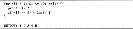
7.2 This problem shows how to exit a for loop before it terminates. This is used in code sample 7.3 to stop the inner for loop, which stops the print statement from writing more output to Poe68. csv.
Perl has the command last, which terminates a loop. For example, code sample 7.5 shows a ioop that should repeat 10 times, but due to the if statement, it terminates in the fifth iteration, which is shown by the output.
Take code sample 7.5 and replace last by next and compare the results. Then replace last by redo and see what happens. Guess what each of these commands does and then look them up online.
Code Sample 7.5 The for ioop is halted by the last statement when $i equals 5. For problem 7.2.
7.3 R isobject oriented (00), and many statisticaloperations produce an object, including lmO. In00 programming, working with objects is done with methods, which are functions. Here we consider the method summary C). Try the following yourself.
Output 7.14 Regression of counts for the as a function of counts for and in the 68 Poe short stories. For problem 7.3.
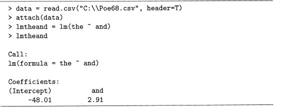
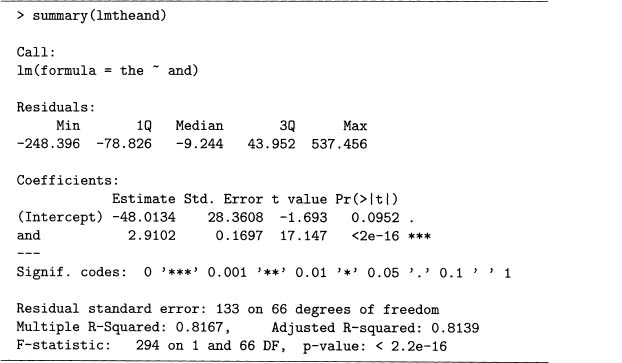
Output 7.14 performs a regression where the counts of the are fitted as a function of the counts of and in the 68 Poe short stories. Compare these results to output 7.2, which is a similar analysis. Here lmtheand is an object, and typing it on the command line gives a little information about it. However, the function summary () provides even more, as seen in output 7.15. If you are familiar with regression, the details given here are expected.
If you investigate additional statistical functions in R, you will find out that summary () works with many of these. For example, try it with eigenO, though in this case, it provides little information. For another example, apply it to a vector of data.
7.4 At the end of section 7.2.4, it is claimed that the correlation matrix is a rescaled version of the covariance matrix, which can be shown by doing the following. First, divide the first row and column by the standard deviation of the first column of M, which is 8.305549. Second, divide the second row and column by the standard deviation of the second column of M, which is 18.70065. Do the same for the third and fourth rows and columns of M using 15.03092 and 14.57738, respectively.
This is also possible by using matrix methods. Convince yourself that output 7.16 is doing the same rescaling described in the preceding paragraph by doing the following steps.
Output 7.15 Example of the function suinrnary() applied to lmtheof from output 7.14 for problem 7.3.
Output 7.16 Rescaling the covariance matrix by the standard deviations of the columns of the term-document matrix M for problem 7.4.
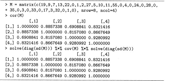
a) First, enter matrix M into R and compute sd(M) . Applying diag() to this matrix selects the diagonal entries. Applying solve 0 to this result replaces the diagonal entries by their inverses. Confirm this.
b) What happens to coy (M) when the following command is executed? Confirm your guess using R.
solve(diag(sd(M))) %*°h cov(M)
c) What happens to coy (M) when the following command is executed? Confirm your guess using R.
cov(M) %*% solve(diag(sd(M)))
d) Combining the last two parts, convince yourself that the following command equals cor(M).
solve(diag(sd(M))) °h*% cov(M) °h*% solve(diag(sd(M)))
7.5 [Mathematicall If matrix M has entries mi jand N has entries Nij, then matrix multiplication can be defined by equation 7.37. Here (MN)i j means the entry in the ith row and jth column of the matrix product MN.
(7.37)![]()
Taking a transpose of a matrix means switching the rows and columns. Put mathematically, ATij equals Aji. Hence the transpose of a matrix product satisfies equation 7.38.
(7.38)![]()
Since equation 7.38 holds for all the values of i and j, we conclude that equation 7.39 is true. If this reasoning is not clear to you, then look this up in a linear algebra text, for example, Gilbert Strang’s Linear Algebra and Its Applications [113].
(7.39)![]()
7.6 The order of matrices in matrix multiplication is important. In some cases, different orders cannot be multiplied. In others, different orders can produce different results. This is easily shown by trying it with some specific matrices. See output 7.17 for an example using the matrices defined in equations 7.40 and 7.41.
(7.40)![]()
(7.41)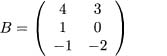
Output 7.17 Example of multiplying two matrices in both orders and getting different answers. For problem 7.6.
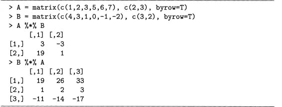
In this case, AB is a 2 by 2 matrix, while BA is a 3 by 3 matrix. So these two products are not even the same size, much less identical matrices.
a) Let M1 be a four by four matrix with every entry equal to 1, and call the diagonal matrix in output 5.5,M2. Compute the matrix products M1 M2 and M2M1. How do these differ?
b) Let M3 and M4 be defined by equations 7.42 and 7.43. Show that M3M4 andM4M3 give the same result.
(7.42)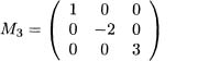
(7.43)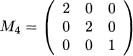
c) Let M5 and M6 be defined by equations 7.44 and 7.45. Show that M5M6 and M6M5 give the same results.
(7.44)![]()
(7.45)![]()
In general, matrices rarely satisfy AB = BA. If they do, they are said to commute. To learn what conditions are needed for two matrices to commute, see theorem 4.15 of section 4.7 of James Schott’s MatrixAnalysisfor Statistics [1081.
7.7 [Mathematical] Equation 7.46 is a two by two rotation matrix, which rotates vectors θ degrees counterclockwise.
(7.46)![]()
a) Verify that equation 7.46 satisfies equations 7.34 and7.35.
b) Compute equation 7.46 for θ equal to 0°. Does the result make sense, that is, does it rotate a vector zero degrees?
c) If equation 7.46 is applied to a specific vector, then it is easy to check that it really is rotated by the angle 6. Do this for 6 equal to 45° applied to the vector (1, 1)T
d) Equations 7.47 and 7.48 shows two rotation matrices. Multiplying M1M2 produces a rotation matrix with angle θ1, + θ2, which is given by equation 7.49. First, show that M1M2 equals M2M1. As interpreted as rotations, does this make sense? Second, the matrix product M1M2 must equal M3, so each entry of the matrix product equals the respective entry of M3. Compute this and confirm that the results are the angle addition formulas for sines and cosines.
(7.47)![]()
(7.48)![]()
(7.49)![]()
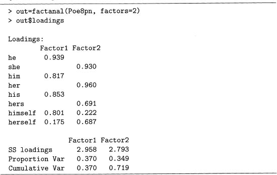
7.8 This problem shows how to do a factor analysis (FA) in R using the Poe8pn data set. This requires specifying the number of factors beforehand. Output 7.18 has two factors, while output 7.19 has three. Although the factor loadings are a matrix, the default is to not print the values below 0.1. Also, the default rotation of fact anal 0 is varimax, so it is used here.
Output 7.18 Example of a factor analysis using the Poe8pn data set used in the PCA of output 7.13. For problem 7.8.
Output 7.19 Example of a factor analysis with three factors. For problem 7.8.
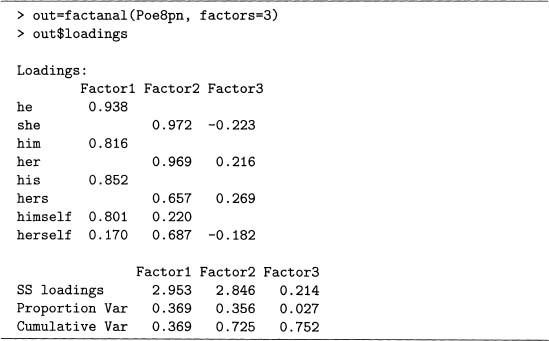
Note that the first two factors for both models have nearly identical loadings. Recall that PCs are interpreted by considering which variables have large coefficients in absolute value, and the same idea is used for factors. Therefore, factor 1 picks out all the male, third-person pronouns, while factor 2 picks out all the female pronouns. Because the PCA performed in output 7.13 shows that PC2 also contrasts pronouns by gender, there are similarities between this FA and PCA.
For this problem, compute a third model with four factors. Compare the proportion of variability for the factors compared to the principal components of output 7.13. Finally, are there any other similarities between the features revealed by the factors and those by the principal components besides gender differences?