Chapter 7

Perturbation Models for Stability, Phase Noise, and Modulation

The complex dynamics of coupled-oscillator arrays lead to the existence of a multitude of steady-state solutions. In addition to finding or selecting a desired steady-state solution, one further needs to guarantee its stability. In this section, perturbation methods are described that allow the designer to examine both the existence and the local stability of the various steady-state solutions of coupled oscillator arrays. An introduction to stability analysis of nonlinear dynamical systems is presented [94], followed by its application to coupled oscillator systems [95, 96].

The perturbation nature of noise, leads to phase-noise analysis methods that are closely related to the formulation used in the stability analysis. Analytical models are presented that demonstrate the attractive properties of coupled inter-injection locked oscillator systems, among them improved phase-noise performance compared to single elements [97].

A straightforward application of coupled-oscillator arrays has been in power-combining arrays where, by controlling the phase shift within an array of synchronized oscillator elements, one can direct the radiated beam toward a desired direction taking advantage of free-space power combining and eliminating the use of lossy power-combining networks. The simple topologies associated with such arrays have led to their consideration in communication system applications where one introduces modulation into the oscillator signals [98, 99]. Thus, methods to introduce modulation in such arrays are presented. These architectures are distinguished from mixer-oscillator arrays where the modulation is not applied in the oscillator signal. Finally, an introduction to the analysis of coupled phase-locked loops is provided.

7.1   Preliminaries of Dynamical Systems

We have demonstrated in Part I of this book that coupled-oscillator arrays are able to synchronize in frequency while maintaining a fixed distribution of the relative phases between their elements and that, despite the complex nature of their dynamics, there are simple methods to control the phase relationships among the array elements, which require a small number of control parameters. It was also demonstrated that as the number of elements increases, there exist many different synchronized solutions, with different ensemble frequency values and different phase distributions. In order to be able to study the behavior of the various solutions as selected parameters of the array are varied, we must first provide a theoretical framework from nonlinear dynamical system theory. This will allow us to classify the types of the solutions and the phenomena that lead to creation or elimination of solutions as well as to changes in the solution stability.

In this section, principles of stability analysis of nonlinear dynamical systems are presented. The theory can be found in standard literature on dynamical systems [100, 101] and nonlinear differential equations [94].

Following Parker and Chua [101] an autonomous continuous time dynamical system is described by the system of differential equations

where the N-dimensional vector contains the state variables of the system, and is the vector field describing the dynamics of the system. The order of system Eq. (7.1-1) is N. An initial condition x(t₀) = x₀ is assumed, where typically t₀ = 0 is set, since the vector field does not depend explicitly on time.

In contrast, a nonautonomous continuous time dynamical system is described by a system of equations of the form

where the vector field depends explicitly on time. A nonautonomous system with period T can be expressed in the format of Eq. (7.1-1) by extending the state vector by one more dimension θ defined by = 2π/T, with θ(t₀) = 2πt₀/T. In the following a dynamical system defined by Eq. (7.1-1) will be considered. A solution of Eq. (7.1-1) for a given initial condition is called a trajectory or orbit.

A free-running oscillator and a coupled-oscillator array are autonomous dynamical systems. They become nonautonomous when an external injection source is present.

A steady state is the asymptotic behavior of a dynamical system governed by (7.1-1) when t → ∞, when the transient behavior has decayed to zero. A steady state is also called a limit set. The mathematical definition of a limit set includes the asymptotic behavior of a dynamical system both as time progresses forward (t → +∞) and backward (t → −∞), distinguishing between ω-limit sets and α-limit sets, respectively.

Steady states can be classified into four different types, equilibrium points, periodic solutions, quasi-periodic solutions, and chaotic solutions.

Equilibrium points x₀ correspond to the solution of

An equilibrium point is the DC solution of an oscillator circuit.

A periodic solution x₀(t), is a solution of Eq. (7.1-1) that has a minimum period T, such as

for every t. A periodic solution of an autonomous system is also called a limit cycle.

A quasi-periodic solution is a solution that is equal to a countable sum of periodic solutions with noncommensurate periods, in other words:

where h_i(t) are periodic solutions with minimum period T_i. The various frequencies f_i = 1/T_i form a linearly independent set of dimension p with 1 < p ≤ M.

Finally, any bounded steady-state behavior that cannot be classified in one of the previous types is a chaotic steady state.

An N-dimensional dynamical system can be efficiently analyzed using a Poincaré map [101, 102]. The Poincare map is a transform that maps an N-dimensional continuous system to an (N − 1) dimensional discrete time system. This is illustrated in Fig. 7-1. Let us consider a continuous-time autonomous dynamical system described by Eq. (7.1-1), which has a periodic solution denoted by L. At some point x₀ of the periodic orbit, we define locally a cross-section Σ that is a surface of dimension N − 1 intersecting L at a nonzero angle. The periodic orbit returns to the point x₀ on the cross-section Σ every T second. The sequence of points on the cross section defines a discrete time system, which is equivalent to the original continuous-time system. Furthermore, the limit cycle of an N-dimensional dynamical system is represented by a point on an (N−1)-dimensional surface. The reader is referred to the literature for a precise mathematical definition of a Poincare map for both cases of an autonomous and a nonautonomous system [101, 102]. It should be noted that the computation of a Poincaré map for autonomous systems is complicated by the fact that the period of the limit cycle is not known a priori; whereas in the case of nonautonomous systems, the sampling period T is known in advance due to the explicit dependence of Eq. (7.1-2) in time.

Having provided the fundamental definitions related to dynamical systems, along with the various types of existing solutions, the stability analysis of these solutions is presented in the next section.

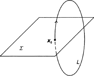
Fig. 7-1. Poincaré map of a periodic orbit.

7.1.1   Introduction to Stability Analysis of Nonlinear Dynamical Systems

There exist different types of stability. For the precise mathematical definitions and types of stability, the reader is referred to the literature [94, 101]. For the purposes of this work, a rather qualitative definition is provided. A steady state x₀ is (Lyapunov) stable if and only if there exists a neighborhood V of x₀ such that every trajectory with initial condition x V remains within V at all times t > 0. Furthermore, a steady state is asymptotically stable if and only if there exists a neighborhood V of x₀ such that every trajectory with initial condition x V reaches arbitrarily close to x₀ given enough time t > 0. In other words, the ω-limit set of any initial condition within V is x₀. Conversely, a steady state x₀ is unstable if there exists a neighborhood V of x₀ such that x₀ is the α-limit set of all initial conditions in V. Finally, a steady state x₀ is called non-stable if for every neighborhood V, there exists at least one point whose ω-limit set is x₀ and one point whose α-limit set is x₀.

7.1.2   Equilibrium Point

The stability of an equilibrium point x₀ is examined by considering the linear perturbation of the vector field f(x) at x₀. The eigenvalues of the Jacobian J(x₀) of the vector field determine the stability of the solution.

with δx(0) = δx₀ representing an initial perturbation from x₀. The solution of the linear differential equation Eq. (7.1-6) generally takes the form

where λ_i and α_i are the eigenvalues and eigenvectors of J(x₀), respectively. The constants c_i are determined by the initial condition δx₀.

For a given N-dimensional vector field f(x) the N × N Jacobian matrix J has N eigenvalues. An equilibrium point whose eigenvalues do not have a real part equal to zero is called hyperbolic. If all eigenvalues have negative real parts, the point x₀ is asymptotically stable. Correspondingly, if there exists one eigenvalue with a positive real part, x₀ is unstable. Finally, if there exists one eigenvalue with a real part equal to zero, the equilibrium point is non-hyperbolic, a condition that is equivalent to the determinant of J being equal to zero, and the eigenvalues of J are not sufficient to determine its stability.

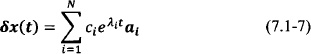
In the case of an (N = 2)-dimensional system, the Jacobian matrix has two eigenvalues λ, which satisfy the following characteristic equation [102]

where σ is the sum and Δ the product of the two eigenvalues. The classification of the hyperbolic equilibrium points and their stability for different values of λ is shown in Fig. 7-2 [102].

7.1.3   Periodic Steady State

In order to determine the stability of a periodic solution x₀(t) the linear perturbation of Eq. (7.1-1), also called a linear variational equation, with respect to the time varying x₀(t) is formed, leading to a system of linear differential equations with periodic coefficients.

with δx(0) = δx₀ and for J[x₀(t + T)] = J[x₀(t)].

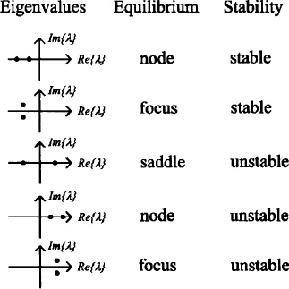
Fig. 7-2. Hyperbolic equilibria of a two-dimensional system.

The solution of Eq. (7.1-6) is derived using Floquet theory [94]

where m_i are the Floquet multipliers and p_i(t) are periodic vector functions. The Floquet exponents λ_i are related to the multipliers by

It is seen from Eq. (7.1-11) that there is not a unique mapping between multipliers and exponents, as adding to any exponent a complex factor jk 2π/T with k an arbitrary integer results in the same multiplier.

The stability of x₀(t) is determined by the Floquet multipliers m_i. They can be calculated by direct integration of Eq. (7.1-9) for one period T with initial condition δx(0) = I_N, where I_N is the identity diagonal square matrix of dimension N. The result of the integration is the monodromy matrix C whose eigenvalues are the desired Floquet mutlipliers m_i [94].

A periodic solution x₀(t) of an autonomous system has at least one Floquet multiplier with magnitude equal to 1, or equivalently a Floquet exponent equal to zero. Furthermore, a periodic solution x₀(t) is stable if the remaining multipliers have a magnitude less than one (|m_i|<1). Correspondingly, if one multiplier with magnitude larger than 1 exists, the solution is unstable.

7.1.4   Lyapunov Exponents

The Lyapunov exponents are defined as

and can be considered a generalization of both the characteristic eigenvalues of the equilibrium point and the Floquet multipliers of the periodic steady state [101]. In fact, the Lyapunov exponents can be used to determine the stability of quasi-periodic and chaotic steady-state solutions.

One can easily see from Eq. (7.1-7) that the Lyapunov exponents of the equilibrium point correspond to the real part of the characteristic eigenvalues.

Correspondingly, the Lyapunov exponents of the periodic steady state are equal to the natural logarithm of the magnitude of the Floquet multipliers divided by the period of the solution, which is equal to the real part of the Floquet exponents.

7.2   Bifurcations of Nonlinear Dynamical Systems

In practice, a dynamical system described by Eq. (7.1-1) depends on a set of parameters ξ of dimension k , which enter the definition of the vector field:

A parameter corresponds to some circuit control voltage or bias voltage/current or any other physical parameter such as the dimension of a transmission line. As the parameter vector varies, the solutions of Eq. (7.2-1) change. The change of stability of a specific steady-state solution, the creation of new steady-state solutions or elimination of existing ones, as one or more parameters of a nonlinear system vary is called a bifurcation [100, 102]. The corresponding parameter values for which a bifurcation occurs are called bifurcation values. A bifurcation diagram is a plot of a selected state variable(s) corresponding to a limit set versus the system parameter(s). An example of a bifurcation diagram is the plot of the DC voltage at a selected circuit node or the oscillation amplitude versus the external bias voltage of the oscillator. Bifurcations are classified into local and global. Local bifurcations are detected by studying the vector field f in a neighborhood of a limit set. In contrast, local information is not sufficient to detect global bifurcations. Typically in this book we study systems where one parameter is varied (k = 1).

7.2.1   Bifurcations of Equilibrium Points

Let us consider such a continuous time system with one parameter that has a hyperbolic equilibrium point. As the parameter varies, there are two ways that a hyperbolic point can become nonhyperbolic. In the first one, a simple real eigenvalue becomes zero (λ₁ = 0). In this case the system is going through a bifurcation known as fold bifurcation. Fold bifurcation is also known as turning-point or saddle-node bifurcation. In a fold bifurcation the equilibrium point curve presents an infinite slope at the parameter value ξ = ξ₀ where one real eigenvalue becomes zero. This is seen in the bifurcation diagram of a one-dimensional system shown in Fig. 7-3.

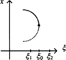
Fig. 7-3. Fold bifurcation.

The infinite slope at ξ₀ corresponding to a real zero eigenvalue leads to a folding, a turning point of the solution curve. For larger values of the parameter ξ > ξ₀ no solutions exist, whereas for ξ < ξ₀ two solutions exist. In fact, one solution branch contains stable nodes indicated by a solid line, whereas the other unstable (saddle) solutions, and this is indicated by a dotted line [102]. In the case of a one-dimensional system, the unstable solution is a node, whereas in the general case it is a saddle. At the critical value ξ = ξ₀, the node and saddle collide, hence the name saddle-node bifurcation.

In the second case, a pair of simple complex eigenvalues fall on the imaginary axis (λ₀ = ±jω₀ with ω₀ > 0). In this case, the system undergoes a Hopf bifurcation, and a limit cycle is born or is extinguished. It is straightforward to see that a Hopf bifurcation requires that the system be at least second order (n ≥ 2).

An example of a Hopf bifurcation in a two-dimensional system is shown in Fig. 7-4. In a supercritical Hopf bifurcation (Fig. 7-4a), a stable limit cycle is born as the parameter goes through the bifurcation value ξ₀. At the same time the stable equilibrium solution becomes unstable. In subcritical Hopf bifurcation (Fig. 7-4b), an unstable limit cycle is created while an unstable equilibrium point becomes stable.

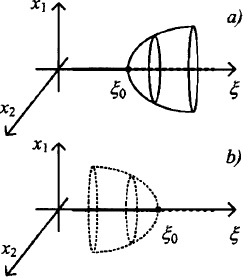
Fig. 7-4. Hopf bifurcation: (a) supercritical, (b) subcritical.

7.2.2   Bifurcations of Periodic Orbits

Correspondingly, a hyperbolic limit cycle is a limit cycle that does not have any Floquet multipliers with magnitude equal to one [102]. A periodic steady state of an autonomous system has one Floquet multiplier equal to one, and therefore, it is hyperbolic if the remaining multipliers do not have magnitude equal to one.

Given a periodic steady state with frequency ω = 2π/T, there exist three types of bifurcations for one-parameter systems [102], corresponding to three distinct possibilities that a multiplier crosses the unit cycle as the parameter is varied, shown in Fig. 7-5.

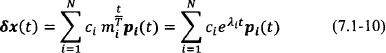
In the fold bifurcation (Fig. 7-5a), a real multiplier takes the value m = 1. In this case the frequency of the limit cycle remains the same, something that can be inferred from Fig. 7-5a) and Eq. (7.1-10), which describes the linear perturbation of the dynamical system around the periodic steady state. A Floquet multiplier equal to 1 leads to a perturbation that evolves as

with n integer and therefore it does not perturb the oscillation frequency of the system. A fold bifurcation leads to a change in the stability of the periodic steady-state solution, much as the fold bifurcation of an equilibrium point does for the equilibrium point.

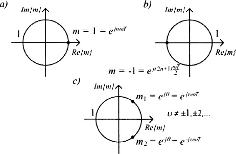
Fig. 7-5. Bifurcations of periodic orbits: (a) fold, (b) flip, and (c) Neimark–Sacker bifurcation.

A flip bifurcation occurs when the multiplier becomes m = −1 (Fig. 7-5b). In contrast to the fold bifurcation, a flip bifurcation leads to the existence of a new limit cycle whose oscillation frequency is half of the original one. Due to this fact, a flip bifurcation is also known as a period-doubling bifurcation. The contribution to the linear variational equation of the m = −1 multiplier is

where one can observe the appearance of a term with a frequency half of the original one.

Finally, in a Neimark–Sacker or torus bifurcation, a pair of complex conjugate multipliers appear on the unit cycle (Fig. 7-5c). As a result, a new frequency, which is not harmonically related to the orininal one, appears in the system, leading to the onset of a quasi-periodic solution. The contribution to the linear variational equation of this Floquet multiplier is expressed as

where ν is not an integer.

7.3   The Averaging Method and Multiple Time Scales

The averaging method is typically used to analyze the periodic steady-state solutions of weakly nonlinear systems

and perturbations of the linear oscillator systems [100, 103], with ε 1. It was originally developed by Krylov and Bogoliubov [104]. The method is particularly suitable to analyze the perturbed linear oscillator problem described by

where ω, x, f . The van der Pol differential equation belongs to this class of systems with f(x) = (1 − x²). In the case of weakly coupled oscillators, an equation of the form Eq. (7.3-2) is used to describe each oscillator, and f(x) contains the nonlinear term of the free-running (uncoupled) oscillator as well as contributions from external coupled signals from other oscillators, which can be linear or nonlinear. The averaging theorem [100] Uc585947 states that there exists a change of coordinates x = y + εw(y, ε), which transforms Eq. (7.3-1) to the averaged system

where

The system given by Eq. (7.3-3) is an autonomous system, whereas Eq. (7.3-1) can be nonautonomous. The essential property of the averaged system that is extensively applied in the study of coupled oscillator systems is that a hyperbolic periodic steady state of Eq. (7.3-3) corresponds to a hyperbolic equilibrium point of Eq. (7.3-1) and that both steady states have the same stability [100]. This essentially means that the eigenvalues of the linearized system of an equilibrium point of Eq. (7.3-3) determine its stability. This is quite useful as obtaining the Floquet multipliers of a microwave oscillator may not be a trivial task. Furthermore, for the cases that are considered in this book, the bifurcations of the averaged system are the same as those of the original system [100].

In order to transform the perturbed linear oscillator problem in the standard form Eq. (7.3-1), the following transformation (known as the van der Pol transformation [100, 103]) is commonly applied to Eq. (7.3-2) before averaging:

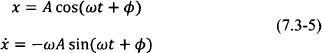
In this case, Eq. (7.3-2) becomes

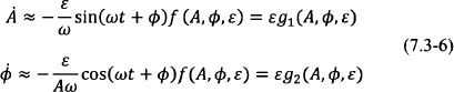
Applying Eq. (7.3-4), the averaged solution is obtained:

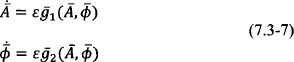
It should be noted that the transformation given by Eqs. (7.3-5) and subsequent application of the perturbation method limits the analysis of the system given by Eq. (7.3-2) locally near the oscillation frequency ω in the frequency domain. The system can be studied near a different harmonic by modifying appropriately the transformation, that is, setting nω in place of ω where n is the desired harmonic order. In practice, considering the oscillator behavior near the fundamental frequency is sufficient for the study of high Q oscillators because higher harmonics are small and therefore can be ignored in the analysis. Specifically, the averaged van der Pol differential equation for which f(x) = (1 − x²) becomes [103]

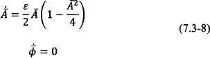
The above system leads to a nontrivial steady-state oscillation with amplitude = 2 obtained by requiring that = 0.

7.4   Averaging Theory in Coupled Oscillator Systems

Kurokawa considered the oscillator equivalent of a series resistance, inductance, capacitance (RLC) resonator connected in series with a negative resistance and applied the averaging theory to study the properties of noisy oscillators and injection-locked oscillators [105].

The theory of Kurokawa applied to the study of coupled oscillator arrays was introduced to the antennas and microwaves communities by Stephan [1] with an aim toward antenna-array applications such as power-combining arrays and phased arrays. The work of Stephan focused on taking advantage of the dynamical properties of coupled oscillator array topologies in order to generate constant phase shift distributions among the array elements in a continuously variable manner. A parallel RLC resonator in parallel with a negative resistance was used to model each oscillator, leading to a dual form of the one used by Kurokawa.

It should be noted that there is significant theoretical work in the literature regarding coupled oscillator systems, also called distributed and ladder oscillators, considering the various operating modes and stability of one- and two-dimensional arrays. Notable references are [106, 107, 108, and 109]. The latter work by Endo and Mori [109] presented an elegant way to obtain a formulation equivalent to a perturbed van der Pol equation in vector form for an array of coupled oscillators modeled as a parallel RLC resonator with a negative resistance, and it will be given in the next section. An efficient analysis of coupled oscillator arrays for quasi-optical power combining and the stability of the various existing operating modes was proposed by York and Compton [110] utilizing only the phase dynamics of the array, or in other words the second equation of Eqs. (7.3-7).

We may distinguish among power-combining applications where the stability of the various operating modes of coupled oscillator systems is with an aim to secure excitation of only the in-phase mode, and applications where an arbitrary phase distribution among the oscillator elements is required (such as beamforming and phased arrays). The latter may be viewed as a generalization of the former.

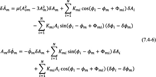
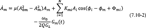
Following their initial work, York produced a general formulation for coupled-oscillator arrays based on the fundamental harmonic approximation and the averaging method that is essentially used to date in most approximate analysis methods for such systems [95, 111]. Furthermore, York introduced an elegant way to achieve constant progressive phase shifts among the array oscillator elements in a continuous fashion by only modifying the oscillation frequency of the end elements of the array. In 2004, Heath presented an elegant and unifying formulation of the application of the method of averaging (specifically the Lindstedt method was used to derive the slow time differential equations [94]) in coupled-oscillator arrays along with a detailed stability analysis of various different coupling network topologies [112]. The latter formulation is given here:

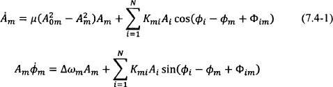
where an array of N oscillators is assumed. The variable A_m represents the slowly varying averaged amplitude of oscillator m, as given in Eqs. (7.3-7) with the bar suppressed for simplicity. Correspondingly, the phase of oscillator m is given by where is the averaged time-varying component of the oscillator phase corresponding to Eqs. (7.3-7) (with the bar suppressed). When uncoupled to the rest of the array elements, each oscillator m has a periodic steady state with amplitude A_0m and frequency ω_m = ω₀ + Δω_m. Furthermore, each individual oscillator satisfies a van der Pol differential equation of nonlinearity constant ε, which appears in Eqs. (7.4-1) through μ = εω_m/(2Q) where Q is the external quality factor of the resonator of each oscillator element calculated using a reference load admittance G_L. Coupling among the oscillator elements is included in the form of a square complex matrix T = [t_mi] of dimension N, with t_mi = T_mie^jΦ_mi. Note that T is a transfer function (unitless). If, for example, an admittance matrix is used to express the coupling among oscillator elements, then T is the admittance matrix normalized to the reference load admittance G_L. In Eqs. (7.4-1) the coupling coefficients also appear in normalized form setting:

Finally, Eqs. (7.4-1) can be written in a complex-valued compact format letting α_m = A_me^j_m:

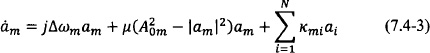
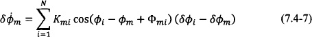
Under weak coupling conditions, the phase dynamics alone are sufficient to analyze the behavior of the coupled oscillator system. We may then consider only the second equation of Eqs. (7.4-1) and assume that the oscillator amplitudes are approximately equal to their uncoupled values A_m = A₀. The system of equations pertaining to the phase dynamics provide significant insight and a very computationally efficient method to analyze arrays with a large number of elements. In fact, the analysis results of Part I of this book have focused on the phase dynamics of coupled oscillator arrays. The system of equations limited to the phase dynamics was introduced as the “generalized phase model” by Heath [112]:

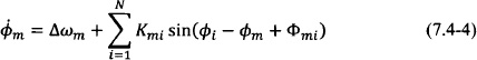
When no coupling phase Φ_mi is considered, the model is the well-known Kuramoto model [113]. In the special case where a bidirectional symmetrical coupling matrix with κ_im = κ_mi is considered, the generalized phase model coincides with the phase model introduced by York [111].

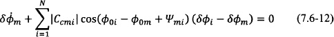
A fixed point of Eq. (7.4-1) corresponds to a periodic steady-state solution, defined for and with c an arbitrary constant. Letting c take nonzero values still corresponds to synchronized solutions of the array but for a different frequency than ω₀.

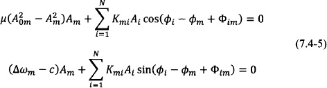
Every set (A_m, _m) that satisfies the above conditions corresponds to an oscillating mode of the array. In principle, there exist up to 2^N−1 modes [111]. It should be emphasized that, due to the autonomous nature of the coupled oscillator system, it is possible to translate all oscillator phases _m by the same arbitrarily large value and still obtain the same steady-state solution. This is evidenced by the fact that only phase differences appear in Eqs. (7.4-5). In other words, the steady state is defined by the oscillator phase differences and not their absolute phase.

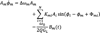
The stability of the oscillating modes is examined by considering the linear perturbation (A_m + δA_m, _m + δ_m) of Eqs. (7.4-1), which leads to a system of linear differential equations:

In the case of the generalized phase model, one has

Because the steady state is defined by phase differences and not absolute phase values, the perturbation phase values δ_m of the steady state may not be small. Their differences, however, are assumed to be small, and this allows one to take the linear approximation of the cosine and sine terms in Eqs. (7.4-1) and obtain Eqs. (7.4-6).

7.5   Obtaining the Parameters of the van der Pol Oscillator Model

A useful analytical method is presented, that allows one to obtain the van der Pol differential equation from a parallel resonator with a nonlinear voltage dependent current source. The procedure follows the development presented by Endo and Mori [108], and it represents a time-domain formulation of van der Pol’s model described in Section 1.2. This model has very low complexity, and it can be easily incorporated into analysis of large arrays or proof of concept for various topologies of coupled oscillators. In addition, it can be easily introduced into circuit simulators.

Given a nonlinear voltage-dependent current source i_n = f(ν) with time derivative di/dt = g_ν(ν), where g_ν(ν) = df(ν)/dv is a nonlinear conductance, and applying Kirchhoff’s current law in the circuit of Fig. 7-6, one has

which, after differentiating, becomes

Defining the natural frequency of the tank = 1/LC, setting ε = g_L/(Cω₀), and scaling time t = ω₀τ the differential equation takes the form

where (   )′ indicates the scaled time derivative d/dτ.

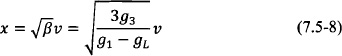
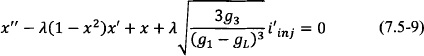
If we consider a nonlinear current source modeled by a third-order polynomial, the equation corresponding to the free-running oscillator (i_inj = 0) can be transformed to the van der Pol equation. Let a voltage-dependent current source be of the form

so that

Setting

one obtains

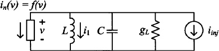
Fig. 7-6. Oscillator model consisting of a parallel RLC resonator and a nonlinear voltage-dependent current source.

The parameter λ is equal to the inverse of the loaded quality factor, Q, of the oscillator circuit of Fig. 7-6.

Finally, scaling the voltage as

the differential equation takes the desired form

When no injection signal is present, i_inj = 0, and this equation becomes the well known van der Pol equation.

The approximate solution to the van der Pol oscillation is [94]

which is identical to the solution provided by the averaging method in Section 7.3.

The approximate parallel model for the oscillator can be extracted using a nonlinear simulator and calculating the admittance at a selected circuit node [114]. Several authors have proposed experimental techniques to evaluate the model parameters [114, 115]. Measurement of the oscillator amplitude can be used to obtain the scaling parameter β. Injection locking the oscillator to an external signal and measuring the locking bandwidth can be used to estimate the Q and subsequently the second parameter λ of the van der Pol model [114]. Alternatively, a low-frequency sinusoidal modulating signal can be introduced in the bias circuitry of the oscillator, resulting in a phase-modulated oscillator output. The parameter λ can then be obtained by measuring the relative amplitude of the modulation sidebands [115].

7.6   An Alternative Perturbation Model for Coupled-Oscillator Systems

It is possible to formulate an alternative practical model for analyzing coupled oscillator arrays by considering that the periodic steady state of the coupled system is a perturbation of the free running steady state of the individual oscillator elements when they are uncoupled to each other. This assumption holds when the coupling is weak, as is typically the case when designing such systems. The model described in this section was proposed in Ref. 116.

An advantage of this formulation is that there is no underlying assumption about the oscillator nonlinearity model, such as for example a third-order nonlinearity used in the van der Pol model, and each individual oscillator can be designed using any numerical technique. The uncoupled free-running steady state is expressed in the slow time (at the fundamental frequency component) as

where Y₀ is the admittance looking into a properly selected node of the circuit and V₀ is the oscillation amplitude at that node (Fig. 7-7).

This is merely application of Kirchhoff’s current law at the node under consideration. Y₀ typically contains both linear and nonlinear terms and depends on the oscillation frequency ω = ω₀ and amplitude V = V₀. Generally, one may assume that Y₀ depends on a number of additional circuit parameters, such as bias voltages. In Eq. (7.6-1) a single parameter μ = μ₀ is considered which corresponds to some DC voltage that allows for frequency tuning. Assuming a nonzero periodic steady-state amplitude V₀, Eq. (7.6-1) is satisfied for Y₀ = 0. A free-running oscillator is an autonomous system characterized by an arbitrary time reference, which translates in an arbitrary phase reference in the frequency domain. As a result, ₀ = 0 may be set without loss of generality.

A coupled oscillator array of N elements is then described by

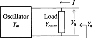
Fig. 7-7. Oscillator 1-port equivalent circuit.

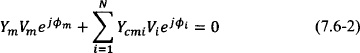
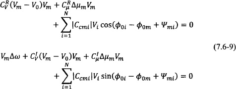
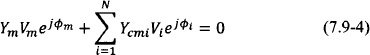
where the coupling is represented by the admittance matrix Y_c(ω) = [Y_cmi(ω)], which typically is frequency dependent. The coupling results in a steady state that can be expressed as a perturbation of the individual oscillator free-running steady state as follows:

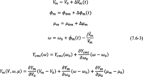
The perturbation assumption has been used in the first place by York, Liao, and Lynch [33], and it is described in Section 1.3 dealing with the injection-locked oscillator. However, in their analysis they proceed to assume a specific nonlinear dependence of the adminttance on the amplitude V_m whereas here no such assumption is made. Furthermore, it should be noted that the frequency expansion has been done using the well-known Kurokawa transformation [105] introduced in Section 1.3. The commonly used coupling networks have a broadband frequency response relative to the oscillator locking bandwidth, which allows us to consider a constant coupling term Y_cmi(ω) = Y_cmi(ω₀). Narrowband coupling networks were studied by Lynch and York [117]. After some straightforward manipulation, one obtains

This system of differential equations represents the basis for an alternative model formulation for a system of coupled oscillators. This formulation has been essentially introduced in Ref. 116 and refined in Ref. 118 as well as in subsequent works as a basis to study several properties of coupled oscillator arrays.

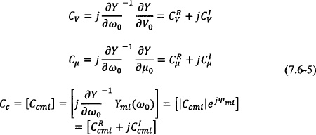
In order to appreciate the similarities and differences with the original model of Section 7.4, the amplitude and phase equations are decoupled by first dividing with and then considering real and imaginary parts. Let for simplicity

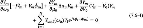
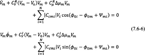
Using the above, Eq. (7.6-4) becomes

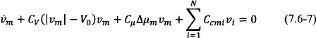
Furthermore, letting ν_m = V_me^j_m it is possible to express Eq. (7.6-6) in a compact complex form:

The corresponding generalized phase model associated with this formulation is obtained considering only the phase dynamics, which results in

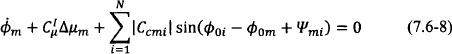
The periodic steady-state solution is obtained by setting _m = 0 and _m = Δω, leading to

or in complex notation

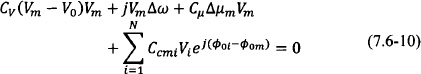
As was the case with the model represented by Eq. (7.4-1) the steady state of the array is defined by phase differences and not absolute phases. In order to study the stability of the steady-state solution, we form the linear perturbation of Eq. (7.6-4) using (V_m + δV_m, _m + δ_m), where small-amplitude perturbations δV_m and small-phase perturbation differences (δ_m − δ_i) are considered leading to

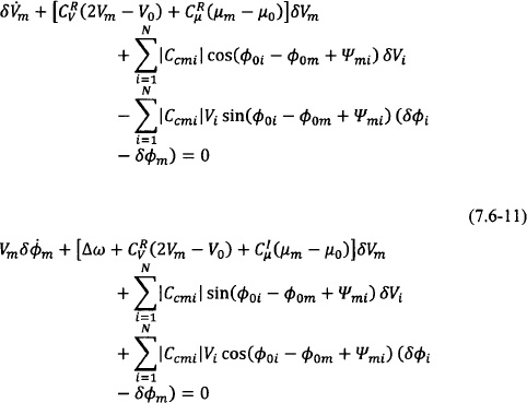
Correspondingly, the generalized phase model stability is then determined by

The eigenvalues of the linear variational equation determine the stability of the steady-state solutions. In practice, it is more computationally efficient to formulate and process the array equations as matrix equations, and this is the topic of the next section.

7.7   Matrix Equations for the Steady State and Stability Analysis

From a computational point of view, it is easier to express the various systems of equations of the previous sections in matrix form. In order to do so, the following notation and properties are used. Bold letterface indicates a column vector or a matrix. The dimension of the vector or square matrix is N unless noted otherwise; 0 and 1 indicate a vector of zeros and a vector of ones, respectively. The notation [a_m] and [a_mi] define a vector and a matrix α, respectively. The function dg( ) converts a vector to a square diagonal matrix of size N. It is straightforward to show that for any two vectors a and b, dg(a)b = dg(b)a. The superscript ( )^H indicates the conjugate transpose of a matrix or vector, whereas superscripts ( )^R and ( )^I; indicate real and imaginary part. One can then rewrite Eq. (7.4-1) in matrix form

where Φ = dg[e^j_m]. The system given by Eq. (7.7-1) can be integrated numerically after separating real and imaginary parts,

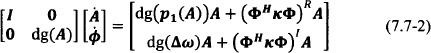
where the vector function p₁(A) is defined as p₁(A) = . The generalized phase model (7.4-4) is then given by

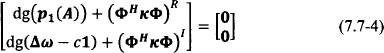
The steady state of Eq. (7.7-2) is computed by setting = 0 and = c1, which, when substituted in (7.7-2), result in the trivial solution A = 0 or

The linear variational equation of Eq. (7.7-1) is also written as a matrix linear differential equation as follows:

with

where g₁(A) = . The complex system of Eq. (7.7-5) is separated into real and imaginary parts as

or

where dg(A)⁻¹ is a diagonal matrix with the inverse of the steady-state oscillator amplitudes in its diagonal. The inversion operation is guaranteed to exist under the assumption that the steady-state solution corresponds to nonzero amplitudes for all oscillators.

Correspondingly, the linear variational equation of the generalized phase model is

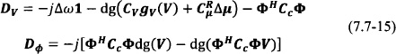
The matrix differential equation pertaining to the coupled-oscillator dynamics according to the alternative model Eq. (7.6-4) becomes

where p_V(V) = (dg(V) − V₀I)V. After separating into real and imaginary parts, one obtains

The steady-state solution is then given by the nonlinear system of algebraic equations

Due to the perturbation assumption, one may consider a linear approximation of the steady state as follows:

For a given frequency offset Δω and phase distribution along the array elements contained in Φ, one may solve the above linear system of 2N equations for the N steady-state oscillator amplitudes and N control perturbations. Alternatively, one may fix the control parameter of one arbitrarily selected oscillator and solve the steady-state system for the N steady-state oscillator amplitudes, the N − 1 remaining control perturbations, and the frequency offset Δω.

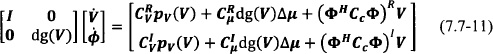
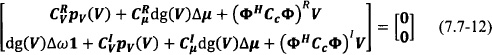
The stability of the steady-state solution is obtained taking the linear variational equation of Eq. (7.7-10), leading to the following linearized system of differential equations:

where

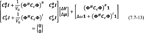
where g_V(V) = 2V − V₀I. One then separates real from imaginary parts to obtain the desired system of linear differential equations:

or

The 2N eigenvalues of the square matrix K determine the stability of the solution. It should be noted that due to the autonomous nature of the coupled-oscillator array, one eigenvalue of K is always zero. The solution is stable if all remaining eigenvalues of K have negative real parts.

One can easily verify that K is unchanged to phase shifts that are common to all oscillators. This is due to the fact that matrix contains only phase differences between the various elements. It is then possible to reduce the system by one, thus eliminating the zero eigenvalue. Selecting an arbitrary element (for example, element j) as a reference, the N phase equations of Eq. (7.7-17) can be reduced by one by subtracting row (N + j), the equation which corresponds to the phase of oscillator j, from every other equation. The equation that corresponds to the phase of oscillator j can then be eliminated. Furthermore, the elements of column (N + j) from row (N + 1) to (2N) are multiplied by zero. In addition, in the amplitude equations, due to the fact that contains only phase differences, it is possible to subtract δ_j from all phases forming . As a result, column (N + j) can also be eliminated because it is being multiplied by zero. The remaining square matrix of dimension N − 1 has the same eigenvalues with K minus the zero eigenvalue. Matrix corresponds to the system of 2N − 1 linear differential equations

where the vector of dimension N − 1 contains phase difference terms relative to oscillator j. The spectral abscissa of a square matrix is the maximum real part of its eigenvalues [119]. Therefore a steady-state solution is stable if the spectral abscissa of is negative.

7.8   A Comparison between the Two Perturbation Models for Coupled Oscillator Systems

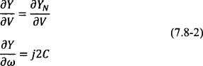
The similarity of the two models is made obvious by comparing the two expressions corresponding to the generalized phase model, Eq. (7.4-4) and Eq. (7.6-8). The first model is defined for a parallel RLC tank with a nonlinear voltage-dependent current source that exhibits a third-order nonlinearity similar to the one described in Section 7.5 and shown in Fig. 7-6. In this case, the admittance looking at the output node of the circuit is given by

where Y_N(V) contains the nonlinear admittance of the current source at the fundamental frequency component. The total admittance contains a real nonlinear admittance term that is amplitude-dependent, plus the load admittance, and an imaginary term which is frequency-dependent. As a result, a real derivative versus the amplitude and an imaginary admittance derivative versus the frequency are obtained:

Furthermore, if we consider that for a parallel resonant circuit the external quality factor is given by

it is straightforward to verify that the Eqs. (7.4-4) and (7.6-8) are identical.

In general, active devices in microwave frequencies exhibit nonlinear susceptance as well as admittance, in addition to a nonlinear admittance that is frequency-dependent. In other words, a more general expression for the admittance at an oscillator circuit node is

As a result, it is possible to view the alternative model (7.6-4) using complex admittance derivatives as a generalized version of (7.4-1).

7.9   Externally Injection-Locked COAs

The coupled-oscillator array is an autonomous system that behaves like a single distributed oscillator. However, there are several applications that require the array to be injection-locked to an external signal. The reason can be to control the phase distribution among the array elements [1], to reduce the array phase noise [97], to fix the array frequency [120], or to introduce modulation to the array [121, 122].

An external injection signal introduces an additive forcing term in the time-domain expression of the perturbed oscillator equation. In Section 7.5, it was demonstrated that the topology of a parallel RLC tank with a nonlinear voltage-dependent current source and an external-injection current term leads to the forced van der Pol equation.

The coupled-oscillator system of differential equations is derived by applying Kirchhoff’s current or voltage law at a selected circuit node or loop of each oscillator circuit in the array. Specifically, in the parallel-tank topology, the corresponding equations are obtained by applying Kirchhoff’s current law at the output nodes of each oscillator. In addition, these nodes correspond to the nodes where the coupling network is connected to each oscillator. However, this does not always have to be the case, and the coupling network may be connected to a different oscillator node.

The external-injection signal typically may not be applied at the circuit node where the coupled oscillator system is derived. In this case it is necessary to derive analytically, or using a circuit simulator, a transfer function, which relates the applied injection signal to an induced current or voltage at the node or loop where the system equation is applied. Alternatively, it is possible to consider that the nonlinear-oscillator admittance is a function of the injection signal. It should be noted that in the general case there may be more than one injection signal applied and that the injection signal may be coupled to the coupled-oscillator array using different topologies, such as direct injection or radiation coupling, as shown in Fig.7-8 [123].

Following the formulation of Chang et al. [123] where the authors assume a parallel resonance model for the oscillator elements, and they consider the external injection signal in the form of an additional current source in parallel with the oscillator tank, one has

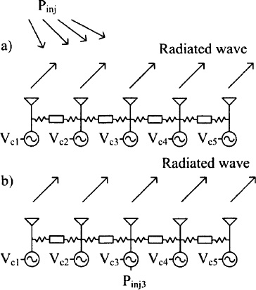
Fig. 7-8. Externally injection-locked coupled-oscillator array topologies: (a) globally injected array and (b) middle element injection.

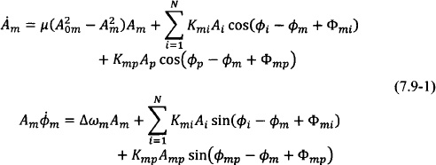
where it is assumed that oscillator m is being injected by an external source mp. The transfer function κ_mp = t_mpω_m/2Q = K_mpe^jΦ_mp consists of a complex normalized term t_mp multiplied with a scaling factor ω_m/2Q as is done for the coupling terms from the other oscillator elements in the array. For the case of an injection-current term in parallel with the oscillator tank, t_mp = 1. Furthermore, when a single oscillator is considered, Eq. (7.9-1) reduces to Adler’s equation.

Alternatively, it is possible to assume that the nonlinear oscillator admittance Y_m(ν_m, ω, μ, a_mp) at the node under consideration additionally depends on the injection signal present at an arbitrary node of the oscillator circuit. Assuming a low amplitude-injection signal relative to the oscillator amplitude ρ_mp = A_mp/A_m 1, a Taylor expansion of the oscillator admittance around the free running steady state gives, to first order [124],

with

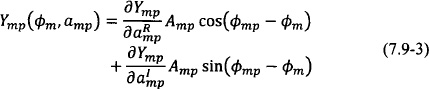
The first term Y_m(V_m, ω, μ) is the one considered in Eq. (7.6-3), where no external injection signal is present. The second term Y_mp(_m a_mp) is a linear perturbation term due to the external injection signal, which depends on the relative phase between the oscillator and the injection signal. The admittance expression is then introduced in the model presented in Section 7.6 and is repeated here for convenience in order to derive the desired system of equations:

As the injection power increases, additional terms in the Taylor expansion can be included in order to improve the accuracy of the approximation [124].

7.10   Phase Noise

Perturbation theory is applied in noise analysis of oscillators as typically noise is modeled as a stochastic forcing term in the oscillator differential equation. The stochastic nature of noise and the nonlinear nature of the oscillator circuits make noise analysis a challenging problem. Applying the averaging theory, Kurokawa [105] presented an elegant analysis of phase noise of free-running and externally injection locked oscillators. A fundamental assumption in his formulation is that noise, described by a time-domain stochastic process n_m(t) can be expanded in a Fourier series around the arbitrarily chosen fundamental frequency ω₀ as

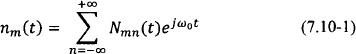
with N_mn(t) = G_mn(t) + jB_mn(t) a complex noise process. In the following it is assumed that n_m(t) is a zero-mean white Gaussian process, which results in G_mn(t) and B_mn(t) being uncorrelated white zero-mean Gaussian processes as well [105].

Extending the work of Kurokawa, Chang et al. [97] studied phase noise in mutually injection-locked coupled-oscillator arrays. Application of the noise expansion and averaging allows us to include the effect of noise in the oscillator formulation Eq. (7.4-1) in terms of N_m1(t) = G_m1(t) + jB_m1(t). In the following, the subscript 1 is dropped for simplicity.

The solution of Eq. (7.10-2) is found in the form of a perturbation (V_m + δV_m, _m + δ_m) where (V_m, _m) is the solution to the noise-free system of Eq. (7.4-1), leading to a forced variational system, which is the same as was considered in the study of the stability of the steady state with the addition of a noise-forcing term. As before, small amplitude-noise perturbations δV_m and small phase-noise-perturbation differences result in the forced linear system of differential equations:

Correspondingly, the alternative model in the presence of noise is modified by including an additive complex noise term N_m(t) = G_m(t) + jB_m(t) in Eq. (7.6-4), which leads to forcing terms G_m(t) and B_m(t) in the left hand side of the first and second equations of Eq. (7.6-11), respectively. For compactness, the formulation is not repeated here.

Following Chang [97], we proceed to solve Eq. (7.10-3) by first applying a Fourier transform

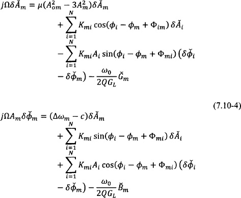
The frequency Ω indicates offset from the fundamental ω₀, and the hat indicates a Fourier transformed variable. The linear system of Eq. (7.10-4) is processed easier in matrix form. Using the formulation of Section 7.7, it is possible to write Eq. (7.10-4) in the form

or

with P = N⁻¹ = [jΩI − D]⁻¹ where the noise terms have been normalized as and for compactness. It should be clarified that the identity matrix in Eq. (7.10-5) is of dimension 2N. Correspondingly, the formulation pertaining to the generalized phase model is

or

with .

The noise correlation matrix S(Ω) of the oscillator array is given by

where the superscript H denotes the conjugate transpose operation. The various noise contributions AM-AM AM-PM, PM-AM, and PM-PM are easily identified.¹ The operator denotes ensemble average, and following Ref. 97 for white Gaussian processes, one has

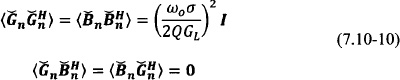
with σ² as the noise variance. Identical oscillators have been assumed and identical noise sources have been applied at each oscillator for simplicity. The spectral density of the oscillator array is given by the diagonal of S(Ω).

The noise correlation matrix is then given by

The generalized phase model expression can be used to obtain an approximate, more simplified expression for the correlation matrix S_G(Ω), without considering amplitude noise:

Note that S_G(Ω) is a square matrix of dimension N containing all correlation terms among the noise quantities of the individual oscillators. The phase noise spectra S_G(Ω) of the individual oscillators in the array are given by the diagonal elements of S_G(Ω), or

The phase noise spectrum S₁(Ω) of a single oscillator element uncoupled to the rest of the array corresponds to D_G = 0 and is given by

This expression is in agreement with the one given by Kurokawa in Ref. 105 and demonstrates the dependence of Ω⁻² of the phase-noise spectrum for the case of white Gaussian noise sources.

The expression for the phase noise spectrum vector S_G(Ω) of each oscillator element in the array finally can be written

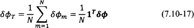
In addition to the phase noise of the individual coupled oscillator elements δ_m, in quasi-optical power combining applications, one is also interested in the phase noise of the combined output of the oscillators δ_T. Assuming small perturbations, one may write the combined far-field amplitude V(t) as [97]

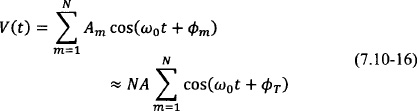
with

The phase noise spectrum S_GT(Ω) of the combined output is given by

which, with the help of Eq. (7.10-15), becomes

Evaluation of the individual oscillator phase noise and the combined output phase noise is generally possible only by numerically evaluating Eqs. (7.10-15) and (7.10-19), respectively. Nonetheless, Chang et al. [97] were able to analytically study several cases commonly found in the literature.

One of the results obtained by Chang et al. [97] corresponds to the case where , repeated here for convenience, is a symmetric matrix . As one can see, D_G depends both on the coupling network, through κ, and on the steady-state phase distribution of the various oscillator array elements, through Φ. It can be easily verified that D_G1 = 0, which reflects the fact that the steady state is unchanged to within a common constant phase term added to all oscillator elements, or, in other words, the fact that the steady state is defined by the phase differences of the various elements. Using the above two properties, Chang et al. [97] have shown by analytically evaluating that , which results in

This is an important result indicating that the phase noise of the combined array output is reduced by a factor N compared to the individual free-running oscillator phase noise (as indicated in Section 6.4). It remains to identify under which conditions D_G is symmetric. One characteristic example is when an in-phase steady-state solution is assumed (Φ = I) and a reciprocal coupling network matrix with zero coupling phase is κ^T = κ = κ^R.

In the case of a reciprocal coupling network of near-neighbor bilateral coupling with zero coupling phase, D_G is symmetric for any constant phase distribution among the oscillator elements. It was also shown that in this case the individual oscillator phase noise is also reduced by a factor N when the oscillators are in-phase. The oscillator phase noise for steady states with phase distributions with nonzero progressive phase Δ_p degrades with increasing Δ_p up to the point where the array loses stability and the phase noise becomes equal to the free-running oscillator phase-noise value.

Finally, it was shown by Chang et al. [97] that there is no phase noise improvement in the case of unilaterally coupled oscillators, for both the individual elements and the combined-array output (as indicated in Section 6.4).

The phase noise of externally injection-locked oscillators has been investigated by Kurokawa [105], where it was shown that the injected oscillator phase-noise spectrum follows the phase-noise profile of the injection-locking signal for small frequency offsets near the carrier, and it converges to the free-running oscillator phase-noise spectrum for large frequency offsets. The formulation of Kurokawa [105] was extended to externally injection locked coupled oscillator arrays by Chang et al. [123]. It is straightforward to obtain the formulation pertaining to the externally injection-locked coupled-oscillator arrays by properly including in Eq. (7.10-2) terms due to injection sources as shown in (7.9-1). Chang et al. [123] investigated several topologies including (a) a globally injected linear array and (b) arrays where a different single elements within the array are injected. In summary, the results showed that for small offsets the array phase-noise profile follows the injection-locking source phase-noise profile. However, for large offsets from the carrier the globally illuminated case showed a different behavior than the single-element illumination topology. In the former the phase noise improves with increasing number of array elements, whereas in the latter the phase noise degrades with increasing number of elements. Furthermore, the array phase-noise performance of the single-element injection case improves as one injects an element closer to the array center.

7.11   Modulation

Several authors have considered the use of coupled-oscillator arrays in communication system applications. It is possible to distinguish among (a) architectures where the coupled-oscillator array signal is modulated and (b) architectures employing a coupled-oscillator array as the local oscillator in a multi-antenna up-converting or down-converting transceiver. The first topology has been studied by Kykkotis et al. [99]. Due to the limiting properties of oscillators, modulation formats that lead to large variations in the signal envelope are not recommended as the oscillator dynamics will tend to smooth these variations and introduce distortion. However, constant envelope modulation formats (such as constant phase modulation (CPM) and Gaussian minimum shift keying (GMSK)) represent excellent candidates to be employed in such systems. In Ref. 99, the modulation is applied in the coupled-oscillator array through an external injection signal. Additionally, it is possible to introduce modulation through the frequency-tuning bias voltage of the individual oscillators, as was proposed by Pogorzelski [63].

A formulation based on Eq. (7.9-3) where the effect of the external-injection signal is included in the oscillator admittance was used by Collado and Georgiadis [124] to analyze the performance of such systems as the modulation bandwidth increases. The effect of the modulation on the maximum stable progressive constant phase shift among the oscillator elements was investigated, and it was shown that the presence of modulation leads to a reduction of the maximum achievable scanning range. In Fig. 7-9, the effect of sinusoidal phase modulation in the maximum scanning range of a two-element coupled oscillator array is shown. The maximum stable phase difference between the first harmonics of the two oscillators is obtained using the aforementioned model (denoted by RoM in Fig. 7-9), in good agreement with measurements as well as simulation results obtained using a commercial envelope transient circuit simulator. (The principles of nonlinear-circuit simulation methods, such as the envelope transient, are described in Chapter 8.) In addition, measurements of the maximum phase difference of the second harmonics of the oscillators are presented, and they are compared with the results using the envelope transient simulator. As can be seen from Fig. 7-9, extended scanning range can be obtained by considering the phase variation of an oscillator harmonic frequency rather than the fundamental frequency. Such architectures used to provide extended phase-scanning range are described in Section 8.6.

On the other hand, the use of coupled-oscillator arrays to provide the local oscillator signal in multi-element communication transceivers has been studied by Pogorzelski and Chiha [74] and Pogorzelski [125]. The coupled-oscillator array is used to provide a local-oscillator signal to a mixer with a desired phase distribution in order to appropriately steer the array beam without the need for phase shifters and a complex local-oscillator distributed feed network. In addition, more compact front ends can be implemented employing an array of coupled self-oscillating mixers as was proposed by Ver Hoeye et al. [79].

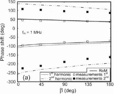
Fig. 7-9. Two-element coupled-oscillator array. Effect of phase modulation index β on stable phase shift among the oscillator elements. Sinusoidal phase modulation of 1-MHz frequency is applied by external injection locking to the one oscillator of the array. The results of the model developed based on Eq. (7.9-3) are denoted by RoM. (Reprinted with permission from Ref. 124, ©2001 IEEE.)

7.12   Coupled Phase-Locked Loops

A phase-locked loop (PLL) is typically used in frequency-generation applications, as well as in phase recovery and phase/frequency modulation/demodulation applications where one oscillator is required to track the phase of a signal present at its input. Therefore, it presents an excellent candidate for generating phase distributions among oscillator elements, which are required in electronic beam-steering applications. Martinez and Compton [126] first proposed the use of a coupled phase-locked loop for phased arrays. Subsequently, Buckwalter et. al. [127] extended their work to study the synchronization properties of such loops, and Chang presented a phase noise analysis [128].

The topology of a coupled PLL system is shown in Fig. 7-10, where a linear array of oscillators is considered. An error signal e is formed by a mixing operation where the outputs of adjacent oscillators are multiplied together. The mixers are used as phase detectors; however, other more sophisticated topologies can also be used where the oscillator outputs are first passed through a frequency divider and are subsequently fed to a digital phase detector, as is typically done in PLL architectures. Finally, the loop is closed by feeding the error signal to each oscillator-control input after it has passed through a loop filter. The relative phases between the oscillator elements are controlled by introducing additional external signals in the error signal path such as x_I and x_N, shown in Fig. 7-10.

In the following, an introduction to the equations describing the dynamics of a two-element coupled PLL system is presented, following the formulation by Buckwalter et al. [127] and based on the topology indicated in Fig. 7-10. Identical oscillators are assumed where, for simplicity, a linear voltage-to-frequency model relation is considered

The index i = 1,2 runs through the set of two oscillators. Furthermore, a first-order loop filter is assumed with gain a, one zero τ_z, and one pole τ_p, having a transfer function given by

Identical loop filters are considered for both oscillators.

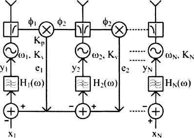
Fig. 7-10. Coupled phase-locked loop architecture.

Based on Fig. 7-10 and considering two oscillators, the following system of equations is derived

It should be noted that for the sake of simplicity the higher-frequency mixing product is not considered in the error signal e₁ as it is assumed that it will be greatly attenuated by the loop filter.

Using the above equations, it is possible to derive one equation governing the dynamics of the phase difference . The external signals x₁ and x₂ can be used to introduce modulation to the loop or simply set some desired phase difference by introducing some offset to the equilibrium point of the loop. Setting external signals equal to zero (x₁ = x₂ = 0), it is straightforward to derive the differential equation so that the phase difference between the oscillators satisfies

where Δω = ω₂ − ω₁ and G = αK_vK_p. The equilibrium points of the coupled PLL correspond to and are derived by solving

It is easy to verify that two solutions exist within the phase interval [0, 2π), and perturbation analysis of Eq. (7.12-8) can be used to show that only the one of the two that falls in the interval [0, π) is stable [127]. This fact implies that the phase difference of the two oscillators for the topology under consideration can be tuned in the range [0, π), by varying the relative frequencies of the two oscillators Δω.

The hold-in range Ω_h of the coupled PLL is the range of the frequency difference among the oscillator elements for which the system remains in a stable equilibrium. The pull-in range, on the other hand, is the range of the frequency difference for which the system will eventually evolve to a stable equilibrium. The hold-in range presents an upper bound to the pull-in range. Based on the above analysis and the stability analysis of the equilibrium points, it was determined by Buckwalter et al. [127] that the hold-in range is equal to

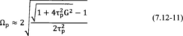
Furthermore, they calculated an approximate value for the pull-in range as given by Eq. 7.12-11 [127]:

Finally, Buckwalter et al. [127] studied the effect of circuit delay on the hold-in and pull-in range of the system. Such delays are present in the system due to the filter characteristics of the circuit, and they result in complex dynamic behavior and instabilities. We remark that such filter characteristics may be fruitfully interpreted as time delays if the delay is small. Unlike Chapter 5 of this book, the analysis of Buckwalter et al. does include the nonlinear behavior. Recall that in Chapter 5 we introduced coupling delay in oscillator arrays via an exponential of the Laplace transform variable. There the analysis was done in the linear approximation, and thus the solutions did not exhibit any of the complex dynamical behavior arising from nonlinearity. The delay introduced was a true time delay due to propagation through the coupling lines and was not constrained to be small. However, the late time behavior in that situation corresponds to solution at time equal to many delay times, a condition which may be satisfied either by large t or small delay or both.

The model described in this section can be made progressively more complex, by taking into account the high-frequency mixing product at the output of the phase detector in the formulation or by using a higher-order loop filter and digital phase detectors.

7.13   Conclusion

In this chapter we revisited the analysis of coupled-oscillator arrays and presented two approximate models that describe the amplitude and phase dynamics at the fundamental frequency of oscillation of the coupled oscillator arrays. We presented a compact matrix formulation of the models, which can be used to efficiently analyze the transient behavior of the arrays, determine the various steady-state solutions, and examine their stability. In addition, we provided a formulation that enables one to consider external injection-locking signals to the array, which can be used to introduce modulation into the array. These models were used to provide an overview of the phase-noise analysis of coupled-oscillator arrays. Such approximate models can be used to simulate large coupled-oscillator arrays in a computationally efficient manner. Finally, it was pointed out that PLLs can be substituted for VCOs in coupled systems, resulting in behavior quite similar to that of the arrays discussed previously. In the next chapter we describe nonlinear simulation methods that can be used to accurately simulate and design oscillator circuits and coupled-oscillator arrays.