Visualizing Risk
In previous chapters, we analyzed market and interest rate risks and generated detailed risk-attribution statistics that decomposed and allocated total measured risk across the portfolio. In this chapter, I hope to provide a basis for thinking about risk and to develop a more rigorous set of risk management tools based upon that thinking. Let's begin by developing conceptually how we see risk geometrically.
Optimal portfolios are all conceptually related in that they provide a risk-minimizing allocation across assets—a set of weights that minimize portfolio risk. Risk, itself, is a weighted average of the individual asset risks as well as their covariances. For example, risk is essentially the sum w′Vw. We have already covered this ground. Covariances are estimated from historical returns that incorporate information about future expected returns and future risks in general; that is, we believe that markets are at least efficient aggregators of information. That is why we think covariances are informative. With this in mind, think of a two-asset portfolio again and the minimum variance portfolio. The minimum variance portfolio is the solution to the familiar quadratic form (usually subject to constraints):
![]()
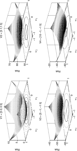
For a two-asset portfolio, this problem can be visualized in three dimensions (x,y,z), where x and y are the two weights and z is the level of risk (dependent on the covariances V and the weights). If we vary weights like we did when we constructed the efficient frontier in Chapter 6, we can show the risk function and conceptualize how the weights are determined that minimize this risk. Figure 11.1 illustrates risk, using four distinct covariance structures. The covariance matrices that these represent are given above each case. V1, for example, represents two assets with identical variances equal to 5 percent but whose returns are independent (zero covariances). This loss surface is symmetric and rises monotonically in the direction of either asset. V2, on the other hand, shows the case in which the returns are correlated which, in general, shifts risk up as measured along the vertical axis, but notice as well that the risk surface loses some of its convexity. V3 illustrates the case in which returns are negatively correlated, thus reducing risks, and V4 shows a case, not unlike the stocks and bonds case in the previous chapter in which one of the asset risks dominates. In this case, the return variance to asset 1 (w1) is three times that of asset 2. The risk contours are projected onto the horizontal (x,y) plain showing how risk changes on the margins as the respective weights are altered. For V4, we see that these trade-offs become more extreme as represented on the ellipsoids—risk is minimized definitely by moving out of the riskier asset.
Figure 11.1 Four Loss Surfaces

I first introduced the optimization problem in Chapter 5, where I wrote out the first order conditions as the derivatives to the quadratic given earlier (with constraints using the Lagrangian). These first order conditions (derivatives) are the gradients, or slopes of tangent planes along these risk surfaces. Imagine, for example, having to try to find the minimum variance portfolio by hand, so to speak. You would start with an arbitrary weight vector—a value for w1 and another for w2. These two weights, with the given covariance matrix, would define a point on the loss surface. You would look at that point, see it was not at the lowest point on the surface, and then change the weights in the direction of the minimum as illustrated in Figure 11.1.
This is how the gradient functions in the computer optimization algorithm we would we using. We compute the value of the gradient using the first order condition and then change the weight vector values in the direction of the gradient toward the minimum (see Figure 11.2
Figure 11.2 Gradient Descent
 ).
).
Constraints such as being fully invested (the weights sum to one) and no short sales restrict the region in weight space that we are allowed to optimize. No shorting would restrict optimization to the positive quadrant while the adding up constraint would restrict it further to weight combinations along the diagonal in the plot in the figure shown here.

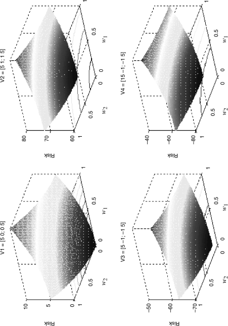
The effects of no shorting relegate the search for the minimum portfolio in the positive quadrant as depicted in Figure 11.3 for these four risk surfaces.
Figure 11.3 Four Loss Surfaces with No-Shorting Constraint

The adding-up constraint requiring full investment (w1 + w2 = 1) basically restricts the search further to a slice perpendicular to the diagonal line given earlier. As such, the region over which the optimal portfolio is found can be seen to be predetermined in large part by the constraints. The gradients we are interested in moving along are in this area as depicted in the next figure (this was constructed using V1).

You can readily see how V4 further pushes the search in the direction away from the high-risk asset and toward asset two (increasing w2 relative to w1 in the process).

As it happens, the minimum variance portfolio for V4 has w2 = 73 percent and w1 = 27 percent. V1 is a 50/50 mix, as are V2 and V3. These last two results may seem somewhat nonintuitive but remember that equal allocations don't necessarily imply equal risk. The risks for (V1, V2, V3) are, respectively (1.58, 1.73, and 1.41), which should make perfect sense to you. The risk on V4 is 1.83.
