Estimating the Hazards of Downside Risks
Monitoring sample movements in the parameters of extreme value distributions are uninformative in that we do not know why a parameter, say, location has shifted further into the tail of the distribution of returns. For this reason, we next devise a hazard function for downside risk conditional on a set of three factors we believe to influence this risk. The hazard rate is the probability of instantaneous failure—the likelihood that a return will exceed the threshold, right now, conditional on the risk state embodied in the values of the risk factors (see Kiefer 1988). We assume the hazard follows an exponential distribution so that the probability of failure is not duration dependent, that is, it is not a function of the length of time elapsed since the last failure; rather it is conditioned only on the level of market liquidity, volatility, and general default risk. There is no reason to restrict the analysis to these three risk factors. We did so for purely illustrative purposes but otherwise encourage more careful study of factors in general. The objective is to attribute the likelihood of extreme returns to changes in factors that we believe drive risks and that we can also observe. Thus, with a forward view on the underlying risk factors, we can form forward views on the probability of failures. A change in this particular risk barometer would, for example, lead portfolio managers to adjust the risk levels targeted in their portfolios if not their allocations. In this section, we demonstrate how such models can be constructed and used to better understand and predict the complex and adaptive return patterns that were depicted in the prior section.
Conditioning the probability of extreme loss on risk factors provides both a model of risk attribution as well as a basis for forecasting downside risk. The hazard model identifies the probability (risk) of a downside event (which we refer to as a fail event) based on the relationship to our three selected risk factors. Because risk factors change daily, our hazard model provides a time-varying probability of instantaneous failure, that is, the probability that the threshold will be exceeded today. See Appendix 13.1 for a discussion of hazard models. The presence of these conditioning covariates can be thought of as shifting the hazard up or down contemporaneously as these variables change. For example, an increasing VIX shifts the hazard up, meaning higher market risks. Our risk hazard model is therefore a probability (λ) of failure conditional on a set of risk factors—the option implied volatility (VIX), the LIBOR spread over Treasuries (TED), and the spread in investment grade credit (AAA corporate rate) over the 10-year Treasury note (DEF) and modeled using an exponential hazard:
![]()
The parameters of the hazard function are estimated by maximum likelihood. Substituting in values for the covariates in conjunction with the parameter estimates gives estimates of the hazard conditional on the respective values for the VIX and the two spreads. This is referred to as the baseline hazard in the survival literature.
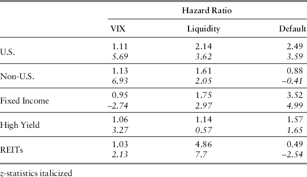
The resulting hazard function coefficient estimates for the five asset classes, pre- and post-Lehman, are presented in Tables 13.4 and 13.5 13.5. For ease of exposition, we report hazard ratios (with corresponding z-statistics in italics). Hazard rates are the exponentiated coefficient estimates, for example, exp(βk) (see Appendix 13.1). A hazard ratio of unity, for example, means that a one-unit change in the risk factor has no impact on the hazard. A hazard ratio of 1.5 means the hazard function rises by a factor of 1.5 for a one-unit change in the risk factor, while a hazard ratio of 0.5 suggests the same change in the risk factor lowers the hazard function by half. Thus, hazard ratios less than unity mean hazard risk falls as the related risk factor rises (and hence the negative z-statistic) while hazard ratios above unity means higher hazard risk for the same change in risk factor. Hazard ratios close to unity mean that hazard risk is relatively unresponsive to the risk factor. From Table 13.4, for the period before the fall of 2008, we can see that for U.S. equity, the default spread has the greatest impact on failure, indicating that a 1 percent increase in the default spread raises the risk of failure by a factor of almost 2.5. For non-U.S. equity, liquidity has the greatest impact; an equivalent increase in the TED spread raises the hazard by a factor of 1.6. All five asset classes have risks relatively neutral to the VIX. REITs have the biggest sensitivity to liquidity with a hazard ratio of 4.86, but for which an equivalent increase in the default spread actually cuts the risk of failure in the REIT market in half.
Table 13.4 Hazard Ratios (data through August 31, 2008)

Table 13.5 Hazard Ratios (data through December 31, 2008)

| Accuracy | |
| U.S. | 76.27% |
| Non-U.S. | 63.64% |
| Fixed Income | 23.68% |
| High Yield | 66.15% |
| REITs | 78% |
Table 13.5 updates the hazard model parameter estimates for the period that includes the last four months of 2008. The changes are economically meaningful and demonstrate the importance of updating the models’ parameters. For U.S. equity, the default spread becomes even more important, completely subsuming the influence of liquidity, now statistically insignificant. On the other hand, downside risk in the high yield market is now very sensitive to default and liquidity.
During the fall of 2008, the default spread, as proxied by DEF, remained at its high through the end of the year while the TED spread fell back to its pre-Lehman level later during October 2008. This may explain why the liquidity factor carries less weight in the full period analysis—fail events and hazards were both peaking by late October as the TED spread was actually declining.
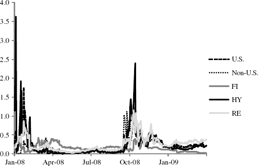
Plots of recursive baseline hazards for the five asset classes are presented in Figure 13.2. The hazard models are estimated over a one-year trailing moving window beginning January 4, 2008, and ending March 30, 2009. The January 4, 2008 hazards are estimated using the prior one year of daily returns and factor observations, and then the oldest observation is dropped as the January 5, 2008 data are added. This one-year window is moved forward through March 31, 2009. One can see a clear transition to higher tail risks across asset classes between September 2008 and October 2008, and declining thereafter but with resurgence in early 2009 as equity markets reached their lows.
Figure 13.2 Baseline Hazards January 2008 to March 2009

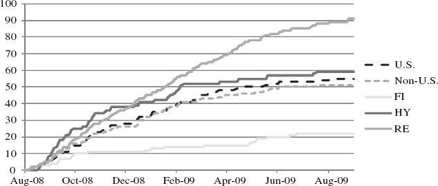
Alternatively, we can observe cumulative fail events across asset classes. These are given in Figure 13.3 as the observed sums of threshold exceedances, beginning August 30, 2008, and ending September 30, 2009. By the end of 2008, REITs and high yield (HY) had the highest incidences of failure and all but REITs tended to moderate in 2009. REIT tail losses continue to accelerate throughout the spring of 2009 ahead of their baseline hazard (see Figure 13.2).
Figure 13.3 Cumulative Hazards

The question remains: How good are these baseline hazards at forecasting fail events? This is a difficult question to answer because baseline hazards do not provide point estimates that give exact failure dates. For the exponential distributions, the expected time to failure E(T), or duration until the threshold is breached, is equal to the reciprocal of the hazard λ(t, x, β) estimated in equation (3). Thus, E(T) = 1/λ. A baseline hazard of 10 percent, therefore, suggests a spell of 10 days until the next failure event. In the case of the exponential hazard, the variance is also equal to 1/λ, and therefore, the exponential has standard deviation of (1/λ)1/2. To get an idea of predictive power, we selected for each asset class all the days from January 4, 2008, through March 31, 2009, on which a fail event occurred. As investors, we care about forecasting the time to failure for the next such event. Thus, for each of those days, we compute E(T) from that day's baseline hazard estimate and find the difference between duration predicted by the model on that day and the subsequent observed duration until failure. There was, for example, a fail event (threshold exceedance) in U.S. equity on January 4, 2008. The baseline hazard updated using the data through January 4, 2008, predicted the next event to occur in 10 days, indicating a standard deviation of ![]() . The observed duration turned out to be seven days, which showed that the prediction was three days too long but still well within a 2-sigma band (the error –3 days was less than –2∗
. The observed duration turned out to be seven days, which showed that the prediction was three days too long but still well within a 2-sigma band (the error –3 days was less than –2∗![]() ). There were 59 threshold exceedances for U.S. equity between January 4, 2008, and March 31, 2009. Of these, the baseline hazard predicted 76.27 percent of the subsequent durations to failure, that is, the observed durations lie within 2-sigma of E(T) estimated from the previous failure date. Note that these results do not use revised baseline hazards. Revisions would imply that if, for example, the observed duration was 14 days from the current failure, we would get to revise our baseline hazard 13 more times until that event occurred. This was not the case. We forecast instantaneous durations conditional on information available on the current day and therefore represent unrevised forecasts. We summarize these results in Table 13.6.
). There were 59 threshold exceedances for U.S. equity between January 4, 2008, and March 31, 2009. Of these, the baseline hazard predicted 76.27 percent of the subsequent durations to failure, that is, the observed durations lie within 2-sigma of E(T) estimated from the previous failure date. Note that these results do not use revised baseline hazards. Revisions would imply that if, for example, the observed duration was 14 days from the current failure, we would get to revise our baseline hazard 13 more times until that event occurred. This was not the case. We forecast instantaneous durations conditional on information available on the current day and therefore represent unrevised forecasts. We summarize these results in Table 13.6.
In general, baseline hazard forecasts are more accurate the higher the incidence of threshold exceedance because they condition their likelihood estimates from an increasing incidence of failures. While this is an attractive property, it is also true that for asset classes characterized by a small number of failures, baseline hazards may have a less accurate forecasting record as well as increased incidence of false positives.
To summarize the analysis thus far, EVT is a univariate procedure; its objective is to model the distribution of extreme negative returns and provide some diagnostics on the stability of the distributions of these returns. We use EVT here to monitor tail risks. The baseline hazard, on the other hand, is a multivariate model of time to failure. Its role is to signal the risk of instantaneous failure and help risk managers monitor this particular risk conditional on a set of risk factors. It also provides a forecast of time to failure that can be used to anticipate future fail events. The power of this model depends on factor selection and the asset class itself. Clearly, we have expended little effort on factor selection; rather, our focus is on method. Our primary interest in baseline hazards is to assess the impact on the hazard from changes in risk factors, that is, to conduct sensitivity analysis and to monitor the evolution of these risks through time and across asset classes.
These two methods represent an important extension to the typical, Gaussian VaR model. Moreover, because standard VaR models use Gaussian distributions, VaR estimates change with the standard deviation of the entire distribution of returns and not the downside tail risk that we wish to focus on. Because standard deviation weights all returns equally, it will tend to evolve more slowly in response to realized extreme losses. Thus, standard VaR tends to underweight extreme values just as our attention is necessarily focused on the left tail of the distribution of returns. Contrary to standard VaR, our EVT model adjusts its risk parameters with high frequency in accordance with market dynamics. We then use our EVT scaffolding to build a robust daily risk hazard model with dynamic linkages to the capital markets. The linkages include volatility, liquidity, and default risk, and can be expanded further in future research efforts. With these attributes, our hazard model gives us the relationship between the market environment and the probability that the environment is either entering (or already in) a crisis.
