A Systemic Risk Indicator
We now turn to our main objective, which is to model systemic risk. The importance of systemic risk is well understood; it manifests itself in the form of higher positive correlations between returns, thereby reducing benefits from diversification, which could lead to significant losses. We define a systemic event as the simultaneous failure of numerous markets or asset classes. For our purposes, we settle on a specific definition of a systemic risk event as one in which three or more of the five asset classes fail on any given day (that is, their returns all exceed their respective thresholds). We can also use the markets of countries to define systemic risk. For example, systemic risk could be defined as the simultaneous failure of three countries.
To describe this mathematically, the systemic event, y is a binary dependent variable that takes the value 1 on a day in which there is a systemic event, and zero otherwise. We use a logistic regression to model the relationship between the likelihood of the systemic event, y, conditional on our three covariates: volatility (specifically, the daily growth rate in the VIX as well as its daily change), default risk (AAA spread over the 10-year Treasury), and liquidity (TED spread). See Greene (2002) for an introduction to logit and probit models and Maddala (1983) on general limited dependent variable models. We therefore estimate the parameters of the following logistic function by maximum likelihood (qualitative differences weren't found by using a probit (normal density). Logistic density was chosen because it has fatter tails:
![]()
![]()
The parameters for this equation are estimated using daily data through August 31, 2008, and are presented in Table 13.7. Perfect foresight forecasts are generated through September 30, 2009, and are depicted in Table 13.8. Our intent is to present the model as we would have seen it as risk managers on August 31, 2008. Perfect foresight assumes we know the factors’ values one day forward. Clearly, we do not, but the point here is to illustrate the model and to examine the odds ratios.
Table 13.7 Systemic Risk Index Model.

As with the hazard models, interpretation of the systemic risk model's parameters are easier after exponentiating the coefficient estimates that, in the case of the logistic function, transforms the analysis to odds ratios in which odds refers to the ratio P/(1 – P), where P is the probability that at least three markets simultaneously exceed their thresholds on any given day. In Table 13.7, therefore, we see that by far, the default factor has the greatest impact in determining the probability that three or more of these markets will experience joint extreme returns on any given day. Furthermore, the model suggests that a 1 percent increase in the default spread increases the odds of a systemic event by a factor of eight. Liquidity is also a highly important covariate. A similar 1 percent increase in the TED spread (liquidity) would produce an odds ratio close to three. Changes in the daily growth of the VIX are more benign but nevertheless significant as well.
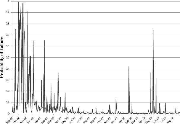
For our systemic risk index, given in Figure 13.4, we estimated the parameters of the logit model as of August 31, 2008, and then predicted the probability of systemic risks going forward conditional on the observed daily values of the three risk factors. The index appears to track well the actual experience, spiking in September 2008, peaking in October 2008, and then tailing off in the fourth quarter only to resurge as the market bottomed in March 2009. One can see the Flash Crash as well in the spring of 2010.
Figure 13.4 Probability of Systemic Failure

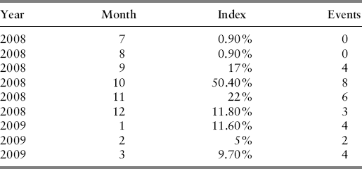
Month-by-month counts of systemic events during the crisis along with the average value of the systemic risk index are summarized in Table 13.8. The risk index reached a peak in October 2008, coinciding with eight systemic events. The default spread in October of 2008 was fully 50 bps higher on average compared to September 2008 and the TED spread (liquidity) jumped from an average of 200 bps to 343 bps over the same period. Even if one could not have forecasted these factor changes, sensitivity analysis based on projections concerning default spreads, liquidity, and volatility would have been very useful in monitoring the likelihood of joint tail risk.
Table 13.8 Systemic Risk Index and Corresponding Systemic Events.

The systemic risk indicator developed here identifies structural changes in markets across a time series of returns and is simultaneously applied to a variety of markets. This high frequency systemic risk indicator reacts in real time to how information and shocks feed back into the evolution of markets. In other words, we effectively explore how stochastic market returns depend on both time and the state of capital markets. In short, this framework provides investors with a picture of the changing nature of risk during crises and provides a valuable guide to helping manage that risk.
