The Efficient Frontier

Now, let's return to our two-asset portfolio. Let's call the expected return to X, r₁, and the expected return to Y, r₂. Let's also refer to the risks on the returns to X and Y as their standard deviations σ₁ and σ₂ with covariance σ₁₂. Suppose that the proportion of the portfolio held in asset Y is a fraction, w, and for X, this fraction is . Then, the return to the portfolio is:

The variance of these returns is

The standard deviation is the square root of this expression. Recall that the definition of the correlation coefficient ρ between the returns on X and Y requires ρ to be a number in absolute value between 0 and 1 and that by definition, . We can use this result to rewrite the variance formula then as a function of the correlation coefficient:

We will use this result to derive the efficient frontier, which is a set of portfolios (of X and Y) that yield the greatest return per unit of risk. Its shape will depend on the returns correlation. First, note we have two equations of interest: one is the return to the portfolio and the other is the standard deviation on the portfolio (the risk). To begin, think of a quadrant in risk-return space and begin by setting ρ = 1, indicating the two returns are perfectly correlated (for example, they are in effect the same asset in this case). Call this Case I. We now have the two equations:

Since we want to work in r,σ space, taking the square root of σ² gives us:

The rate of change in the return and the risk with respect to the portfolio weight is:

Therefore, the risk-return trade-off for Case I is:

Thus, the return-risk trade-off falls along a positively sloping line in the risk-return space. It is positively sloped, since it must be that if r₂ is greater than r₁, then σ₂ must be greater than σ₁. Otherwise, there would be an arbitrage opportunity to sell the riskier asset with lower return and to buy the less risky asset with a higher return and earn an arbitrage profit. Arbitrage profit opportunities cannot persist.

Now assume the opposite limiting case that . Call this Case II. In this case, we have:

Taking the square root of the variance to get the risk relationship, we get the following two equations:

For the risk to be defined (that is, positive), it must be that . When the weight w is small, then this will be the case. Specifically, you can see that as long as

, then this condition is satisfied. When , then the relationship becomes . Call this Case III. Therefore, there is a switching point at which , and substituting this expression into σ, we solve for the switching point:

This is a point in risk-return space. It has zero risk and vertical intercept equal to the value of r just given. I now derive the rest of the efficient set.

We have these two additional cases beginning with Case II:

Case II, therefore, is a line with negative slope. Case III, however, is:

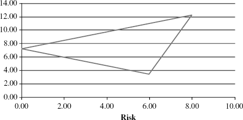
This is an upward sloping line in r – σ space. Putting these ideas together, we derive the general shape of the feasible set of portfolios that can be constructed across these two assets. (See Figure 5.2.)

Figure 5.2 Feasible Set

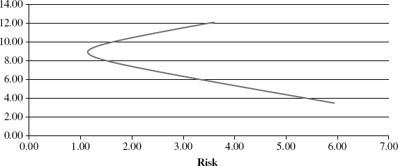
In general, the correlation coefficient between the returns is less than one in absolute value, and the actual value will determine the shape of the feasible set. From the preceding figure, we see that portfolios along the lower boundary are dominated by those directly above them. For example, for two portfolios with the same risk, we'd prefer the one with the higher return. Therefore, the efficient set consists of the top portion of the feasible set. When the correlation coefficient is less than one in absolute value, this frontier is convex. Figure 5.3 shows the feasible set using Figure 5.1, which depicted payouts to two assets, X and Y, which have correlation equal to –0.87.

Figure 5.3 Feasible Set for Contingent Claim Example