Markowitz Portfolio Selection Criteria

Efficiency is about minimizing risk. The efficient frontier is the set of risk-minimizing portfolios for any given set of returns. The mean-variance efficient portfolio is the one with minimum risk. Markowitz's contribution was to give us the calculus to solve portfolio problems like this. The objective is to find the weightings (w_i) that minimize the risk for a given portfolio return. Achieving this would generate a weighting of the assets in a portfolio, which would occupy a point on the efficient frontier. How can one achieve this objective? Consider again the risk we solved earlier and reprint here:

We desire to choose the weightings (the w_i and w_j) that minimize this quantity for a given portfolio return. There are several ways to set up this problem and I outline a few here that serve as a platform for our empirical work in Excel. I begin with a very intuitively appealing representation of the problem as a risk-adjusted return maximization in matrix format that solves for the vector w that maximizes the quadratic form given by:

Here w is a k-dimensional row vector of weights , where k stands for the number of assets in the portfolio, r is a conforming vector of expected returns ( column vector), V is the covariance matrix , and λ is a risk aversion parameter (more on risk aversion later). Thus, is a scalar that measures the return to the portfolio (it is a weighted average of the expected returns) and is a scalar that measures the risk on the portfolio. (This is the quadratic part because it involves the squared values of weights, variances, and covariances. We divide by two to account for the square, which we'll also see more clearly later. For now, understand that its presence doesn't affect the solution). Thus, we want a set of weights that maximizes the risk-adjusted return. A review of matrix operations is in the appendix to Chapter 6.

Differentiating with respect to , setting this expression to zero and solving for the remaining w yields:

The solution w is a vector of weights that define this optimal portfolio. Ignoring the risk-aversion parameter for the moment (this serves only to scale the solution), assume that V is a diagonal matrix, meaning that the returns to the k assets are independent and that the diagonal elements of V are the returns variances. Then the solution is a portfolio whose weights (w) are their respective expected returns divided by their respective variances. The portfolio that minimizes risk chooses assets in proportion to their return per unit of risk, that is, the lowest risk-to-reward ratio.

If returns are not independent, then V contains covariances and the inverse of V is more complicated. Nevertheless, the optimal portfolio still has the same interpretation, only here the risk on each asset extends to the strength of its correlations with the other assets. In general, the more positive those correlations, the higher the risk (bad things can happen to more than one asset at the same time, so to speak) and the lower the weight assigned to that asset. We investigate this more closely in our empirical applications further on.

Let's now break apart the matrix algebra into the set of underlying equations so that we can get a better understanding of what's going on in the calculus. At the same time, let's address a few important constraints like forcing the sum of the weights to equal unity (fully invested portfolio) and that the desired portfolio return is known ahead. How do we do this? We do so by writing the Lagrangian (this is a constrained optimization problem) and using the first order conditions to solve for the weights. We'll set it up formally first and then talk about the intuition. We wish to optimize the following setup, which is to find a portfolio w that minimizes the risk:

Subject to the two adding-up constraints:

and

The first constraint says that the weighted asset means in the fund must sum to the targeted return on the portfolio. The second says that the weights must sum to unity (we say that the fund is fully invested; there's no money left on the table, so to speak).

We now form the Lagrangian:

We differentiate this function with respect to each of the w_i in the portfolio and with respect to the Lagrange multipliers lambda (λ) and mu (μ). That means we will end up with k first order conditions (there are k assets, and therefore one derivative for each) and two derivatives for the constraints for a total of first order conditions. We set each of these first order conditions equal to zero and solve this system of equations simultaneously for the weights as well as λ and μ as the constraint parameters (we'll focus on the weights).

The first order conditions involve k equations, one for each w_i followed by the two constraints.

To make the first of these three relations make sense, think of a two-asset portfolio and the covariance structure of its returns given by:

The diagonal elements are the variances, and the off-diagonal elements, the covariances. The portfolio risk was derived earlier in this chapter. It must be, therefore, that the following two relations are equivalent:

This, incidentally, has the matrix equivalent:

Either way, we can now see that differentiating the Langrangian with respect to the weights produces the following first order conditions:

As promised, there are equations in four unknowns. One solution method is Cramer's Rule; the other is straightforward matrix multiplication, which I prefer to use since this is the method most suited to our spreadsheet work that will follow later. Our system is given directly further on. The data are in the first matrix. The parameters we wish to solve for are in the second vector (w₁,w₂,λ,μ)', while the targeted values in the constraints are in the vector on the right-hand side of the equation.

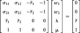
Solving this system is not hard. If we represent it as , then . Our minimum variance portfolio consists of the first two elements in x. The leftmost point on the efficient frontier is the minimum variance portfolio. We can solve this portfolio by eliminating the third row in A, x, and b and the third column in A and solve for (w₁, w₂, μ)'.