Applications and Examples
Example 9.1: The Fama-French Three-Factor Model
Recall that I presented this model as an extension of the CAPM single index model. The factors represent the return premiums on mimicking portfolios constructed on value (HML) and size (SMB) as well as the market portfolio (rm).
![]()
Notice that this is a time series regression (indexed by t) whose parameters are estimated for each stock or portfolio of stocks (indexed by i). This is fundamentally different from the cross-sectional regressions developed in the previous section, as I will make clear shortly.
![]() Go to the companion website for more details.
Go to the companion website for more details.
Chapter 9 Examples.xlsx estimates the parameters of this factor model using the returns on the minimum variance portfolio solved for in Chapter 7. (Because I want to focus on the factor sensitivities, I will ignore the standard errors of the parameter estimates and statistical tests of significance in these examples). Since this portfolio was constructed on 10 large capitalization stocks, it is no surprise that it has a beta close to one with the market portfolio. Here is the model estimated on the first three years of data (through March 1997).
![]()
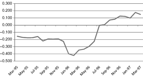
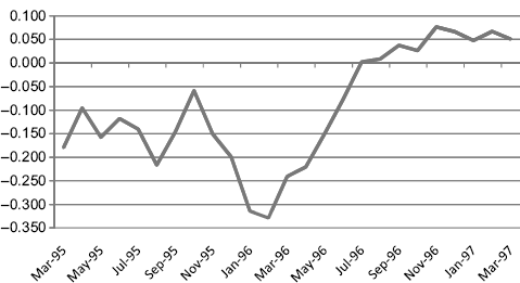
The returns to the portfolio are negatively related to value and small firms as we'd expect; after all, these are large cap growth firms. To get at some dynamics, I rolled these regressions forward in a three-year moving window through March 1997 (see Figure 9.1). As the following charts indicate, the portfolio's style appears to change dramatically over this period leading into the tech bubble of the late 1990s.
Figure 9.1 Fama-French Value (HML)

This portfolio begins to track the value portfolio in mid-1996 and, at approximately the same time, starts to become relatively neutral to size (see Figure 9.2
Figure 9.2 Fama-French Size (SMB)
 ).
).
The style drift we are witnessing here is likely the impact of the runup in tech stocks during this time—earnings-to-price ratios as you will recall, had reached historical highs on the S&P 500 index late in the decade—as some of the firms in this portfolio were beginning to perform more like small value stocks. These data in the spreadsheet extend through 2006, so it is possible to track these factor sensitivities past March 1997. I will leave that as an exercise. One caveat worth mentioning at this point is that the portfolio returns are calculated on the minimum variance portfolio as of March 1995. This portfolio was then allowed to drift and hence the portfolio we are analyzing after this point in time is likely not the minimum variance portfolio. In practice, we would reoptimize, or rebalance, this portfolio periodically. See Chapter 21 on Optimal Rebalancing.
Example 9.2: Macro Factors
This model decomposes an assets's return into four risk-factor contributions. We look at volatility (implied volatility, captured by the VIX index), inflation risk, default risk (AAA corporate spread over Treasuries) and liquidity risk, which is proxied by the TED spread (LIBOR over the 90-day T-bill). Again, this is a time series model. Each asset's return is regressed separately, since there is no informational gain to pooling returns into a panel regression because they all share identical exposures to the risk factors. We therefore estimate the parameters of the following model for asset i using least squares:
![]()
Refer to the second tab on the Chapter 9 Examples spreadsheet to view data and the results. Using the same procedure we used earlier for the Fama-French three-factor model, I estimated the parameters for the same minimum variance portfolio with a trailing three-year window beginning in March 1995.
![]()
This says that the minimum variance portfolio return is expected to fall by 2.723 percent for each 100 basis point increase (1 percent) in the default spread but only 37 basis points (bps) for an equivalent increase in the TED spread. Returns tend to increase with inflation—an effect that is established in the literature but only for moderate and low inflation; high inflation will drive returns down—which is consistent with the claim that equity is a natural inflation hedge. Returns are also predicted to be higher in volatile markets as indicated by the positive sign on the VIX, which also makes sense. Although this effect is weakest in magnitude, keep in mind that the VIX can change a lot compared to the spread instruments. For example, the VIX can go from 15 to 45 in the time it takes the default spread to change by 100 bps. In fact, in our data, the VIX has roughly 25 times the volatility of the default spread.
In either model, we could forecast the asset's return conditional on our views regarding the factors. If, for example, we believed that the default spread was going to tighten by 50 bps over the holding period for this asset, then we might raise our expected return estimate by 1.35 percent. In general, we estimate factor models over all the assets in the portfolio (say, each of the 10 firms comprising these data) and use our views to forecast expected returns, which are then input as arguments in our optimizer. Therefore, given a covariance matrix V and a vector of expected returns conditional on specific factor exposures, we solve the mean-variance efficient portfolio as outlined in Chapters 6 and 7.
Factor models give us some perspective on how asset returns are influenced by and respond to movements in various factors that influence risk and return on the portfolio. They also provide an alternative to using the unconditional mean return, which is, by definition, an equal weighted average of past returns and not necessarily indicative of future returns. If we are confident in the model specification (choice of factors) and the estimates of the factor sensitivities, then the factor model serves as a means to generate more realistic forward returns estimates.
Example 9.3: Fundamental Factor Model
Here is an example that more closely tracks the methodology of the MSCI-BARRA fundamental model. Using monthly data from January 2001 through November 2009, I constructed a panel data set (cross-sectional time series) on the MSCI All World Index for the following major GICS: Energy, Consumer Staples, Materials, Health Care, Industrials, Financials, Consumer Discretionary, Information Technology, Telecommunications, and Utilities.
To keep the model tractable, I selected five fundamental factors. These factors are called fundamental factors since they are factor exposures unique to each sector at each point in time: Dividend yield, value, size, momentum, and volatility.
In each month, each fundamental factor is standardized across the assets in the portfolio, which, in this example, is the 10 sectors. (This example is illustrative. In practice, we would be working with hundreds or thousands of assets for which statistical properties would be much more robust.) Therefore, the estimated factor sensitivities measure the expected response in the asset return, given a one standard deviation change in the fundamental factor. The final data set consists of 107 monthly observations on 10 sectors. We are therefore estimating the k = 5 parameters on t = 1,..., 107 observations.
The methodology requires estimating a cross-sectional regression involving N = 10 observations in each of the 107 months. This is a bit cumbersome in Excel, so I did it in Matlab. The results, however, were written to the tab labeled Fundamental Factors in the spreadsheet. There, you will find first a 107 × 5 matrix of factors sensitivities followed by a 107 × 10 matrix of the conditional expected returns. The covariance matrix V for the betas follows. This example is small enough that we can use it to highlight the power of fundamental factor models in helping us generate the covariance matrix that we need for the mean variance optimization problem. Recall that for large N, this covariance matrix is impossible to estimate from returns data alone. The factor model, however, provides an avenue to arrive at a full-rank covariance estimate, and that matrix is given on the spreadsheet as Vx. Again, I abstract some details for simplicity. In this case, I am ignoring Vε, which is the diagonal matrix of specific risks estimated using the residuals collected from the 107 cross-sectional regressions. Compare this matrix to that estimated using the actual returns, V (which we can do in this example since T is sufficiently large relative to N). The optimizer takes as arguments Vx for the minimum variance portfolio, or Vx, and some expected return vector (from the matrix of estimated factor-based returns) for the minimum variance portfolio with targeted return. It is interesting to see what the minimum variance portfolios would have looked like in both cases. See Table 9.1.
Table 9.1 Minimum Variance Portfolios.
| V | Sector | Vx |
| –0.221 | Energy | –0.249 |
| 0.856 | ConStap | 1.036 |
| –0.786 | Materials | –0.051 |
| 0.162 | HealthCare | –0.142 |
| –0.048 | Indust | –0.143 |
| 0.106 | Fin | 0.269 |
| –0.053 | ConDis | –0.049 |
| –0.009 | IT | –0.108 |
| 0.227 | TeleCom | –0.209 |
| 0.766 | Util | 0.644 |
These are not identical; nor should they be. The fundamental portfolio using Vx is estimated using a covariance matrix that is a function of the last observation on X, that is, XVβX′, with X being the exposures from the most recent month. Therefore, we see that Vx contains a dynamic element not typically present in V by weighting the covariance matrix more heavily on the most recent factor exposures.
Fundamental quant managers will sometimes tilt their portfolios in the direction of certain factors, for example, by estimating expected returns off of a subset of factor exposures and factor sensitivities. On the other hand, they may restrict weights to certain sectors, thereby overweighting the remaining sectors. Overweights to certain sectors are sometimes based on macro factor models like those outlined in Example 9.2, discussed earlier.
