Chapter 3
Protocol Level Spatio-Temporal Processing
3.1 Introduction
Following the rationale behind the autonomically driven cooperative design established in the previous chapter, where a specific umbrella was created with the intention to encompass all the architectural considerations to be outlined across the entire book, the time has come to commence the rollout thereof with the foundations related to protocol level spatio-temporal processing. To this end, first of all, the emphasis is laid on the bottom-most multiple-input multiple-output channel conditioned developments, to provide a good understanding of their workings, and especially to put them in the correct context before they can be properly integrated into the Autonomic Cooperative Networking Architectural Model. Thus, the diversity-rooted origins of the approach based on multiple-input multiple-output technology are discussed, so that it is possible to clearly justify the role of and necessity for the later deployment of spatio-temporal processing enabled techniques on top of it. Before the focus is shifted, however, the question of radio channel virtualisation is addressed, where the singular-value decomposition theorem is explained in order to introduce the notion of an equivalent virtual multiple-input multiple-output radio channel to be deployable among Autonomic Cooperative Nodes. The radio channel capacity is then brought into the bigger picture of the whole analysis to account for its linear scaling with the number of generic transmitters or generic receivers. What is more, an external model for radio channel coefficient calculation, to be employed in the next chapter, is summarised, and the difference between coding gain and diversity gain is addressed for clarity.
The focus then moves towards space-time coding techniques, with the intention of accounting for their superiority over the above-mentioned diversity techniques, especially the possibility of shifting the complexity related to the deployment of multiple antennae on, usually relatively small, mobile user terminals to a base station or an access point, and to pave the way for their later elevation to the level of networked configurations, where the transition towards the concept of distributed space-time block coding shall prevail. In this respect, first of all the most baseline approach to space-time coding, in the form of orthogonal block coded designs, is outlined, with a special emphasis on space-time block coding, where not only the method of operation behind this technology is explained, but the question of its being perceived more as a modulation rather than a coding technique is touched upon. Then the plot is extended even further in this respect, to outline the derivation of the decoding metrics for a selected set of space-time block coding matrices with the aim of building on it in introducing the concept of the equivalent distributed space-time block encoder in the next chapter. This derivation is performed not only to make the related processes of coding and decoding more transparent, but also to clarify certain inconsistencies the author came across in the source materials. Last, but not least, an extension towards space-time trellis coding is presented, where the expected additional coding gain becomes obtainable.
Once all the aforementioned technological aspects, key to the overall Autonomic Cooperative Networking Architectural Model, have been outlined, their mutual relation with the protocol level related control logic is discussed for architectural integration purposes. In this way a specific pattern is created to be followed throughout the entire book to outline an incremental advancement of the proposed design. In particular, this part opens with the introduction of the notion of an Autonomic Cooperative Node being, de facto, one of the major building blocks when the workings of the proposed concept are concerned. On this occasion, not only is the relation between autonomics and cooperation discussed in detail, but the internal structure of such an Autonomic Cooperative Node is scrutinised from the perspective of the Generic Autonomic Network Architecture, so that it is possible to outline the adopted interaction model over the Open Systems Interconnection Reference Model protocol stack. Then, the cooperative transmission decision element is brought into the analysis as being characterised as belonging to the protocol level, while being mostly responsible for the interaction with the routines of the physical layer. Given such a context, not only is the role and notion of the concept of a protocol discussed, but certain adaptive logic is presented where the relevant code matrices are switched on the basis of the radio channel parameters. Finally, all the pertinent architectural integration aspects are outlined, with a particular approach to the graphical representation thereof, and the way is prepared for further extensions.
3.2 Multiple-Input Multiple-Output Channel
3.2.1 Diversity-Rooted Origins
From the scope of this book and the high-level design presented thus far, one could apparently attempt to say, probably without too extensive an exaggeration, that diversity laid the foundations of most of the aspects of the latter, if not all of them, even if it happened more or less directly. In fact, this claim may seem well justified, as not only did this notion generally add new dimensions to the overall perception of multi-path propagation,1 but its evolution inevitably led to the invention of key technologies so crucial to further advancement of the proposed concept, just to mention its influence on spatio-temporal processing (STP) or cooperative relaying, as respectively summarised by Phan et al. (2013) and Liu and Lin (2015). In fact, the rationale behind the introduction of the related gain obtainable thanks to such diversity is deeply rooted in the assumption that multiple replicas of the transmitted signal, as observed by the receiver, convey constructively redundant information, while the fading they shall be subject to may be rather poorly correlated. This way, it could become highly unlikely that all such replicas would encounter a deep fade at the same time, which increases the probability of proper reception. Since there exist numerous approaches in this respect, the most generic categorisation of the diversity techniques of relevance seems to pertain to the domain of their application, and thus it is possible to distinguish generally between temporal diversity (TLD), frequential diversity (FLD), and spatial diversity (SLD) (Wódczak, 2014).2 In this context, the shortlisted techniques will be analysed, and their related developments will be discussed in the light of the upcoming developments.
Looking at the first of these categories, one may immediately identify that, as originally explained by Jankiraman (2004), the role of temporal diversity consists in the transmission of multiple replicas of a signal using disjoint time slots where, according to Vucetic and Yuan (2003), it is mandatory that a separation should exist between the time slots such that its size would be equal at least to the coherence time (CT) of the channel, defined by Goldsmith (2005) as the time during which the autocorrelation function of the channel impulse response is approximately nonzero. Apparently, as such an approach may cause decoding delays, it is said to be mostly suitable for fast fading environments, where the aforementioned coherence time is relatively insignificant. Moving forward to frequential diversity, one may see that this approach assumes, in turn, the exploitation of different frequencies for the very similar task of transmitting replicas of the original signal. As for temporal diversity, such frequencies need to be properly separated, since different parts of the spectrum undergo independent fades (Jankiraman, 2004). To reflect this situation, the relevant separation is denoted by the complementary term of coherence bandwidth (CB), which is defined by Goldsmith (2005) as the frequency range across which the entire signal bandwidth is highly correlated. In other words, also following Vucetic and Yuan (2003), should the fading statistics for different frequencies appear to be essentially uncorrelated, a frequency separation of the order of several times the channel coherence bandwidth would be required for proper operation.
By contrast to the above categories, spatial diversity does not really induce redundancy either in the temporal or frequential domain, as detailed by Vucetic and Yuan (2003); in its case, the constituents of a multi-element array (MEA) are separated by a few wavelengths to guarantee that replicas of the transmitted signal do not become correlated; hence, this type of separation is usually referred to as coherence distance (CD), to follow Jankiraman (2004). What is more, according to both Vucetic and Yuan (2003) and Jankiraman (2004), this category may be additionally extended to encompass two representative approaches to exercising radio transmission diversity in the spatial domain, known as polar diversity (PLD) and angular diversity (ALD).3 In particular, in the case of polar diversity the signals, characterised by being polarised either horizontally or vertically, are transmitted and received by two sets of differently polarised antennae in order to ensure that there is no correlation between such signals, even if the antennae belonging to such sets are not guaranteed to be separated by a distance corresponding to a few wavelengths. As for angular diversity, such an approach is applicable given carrier frequencies of the order of several gigahertz, which are characteristic of environments featuring rich scattering in the spatial domain. Thus, it would suffice to use two highly directional receiving antennae, each facing in a different direction, to fully exploit spatial diversity (Vucetic and Yuan, 2003).
However, given the major theme of this book, it becomes pragmatically justified to provide additional insight into the category of spatial diversity, especially since space-time coding (STC) techniques will be addressed shortly. In essence, depending on whether the MEA is located at the transmitter or at the receiver, two major subcategories, known as reception diversity (RND) and transmission diversity (TND), may be distinguished.4 In fact, as explained by Vucetic and Yuan (2003), one of the least sophisticated approaches to reception diversity is selection combining (SC), outlined in Figure 3.1, where a given signal is preferred should it be characterised by the highest value of the instantaneous signal-to-noise ratio (SNR), which obviously requires that all the diversity branches be monitored simultaneously. Therefore, the suboptimal solution of switched combining (SWC) or scanning diversity (SCD) was introduced, where that diversity branch remains selected which is able to maintain the SNR above a specified threshold. Moreover, there is the linear method of maximal ratio combining (MRC),5 as depicted in Figure 3.2, where distinct diversity branches are weighted with the use of ![]() coefficients and then submitted to the superposition module. In this case, the
coefficients and then submitted to the superposition module. In this case, the ![]() coefficient may be written as
coefficient may be written as
where ![]() is the amplitude and
is the amplitude and ![]() is the phase of the received signal
is the phase of the received signal ![]() observed at antenna
observed at antenna ![]() , so that the overall received signal
, so that the overall received signal ![]() may be expressed as
may be expressed as
As additionally analysed, for example by Vucetic and Yuan (2003), maximal ratio combining is an optimum combining method from the perspective of the maximisation of the SNR at the output.

Figure 3.1 Selection combining. Adapted from Vucetic and Yuan (2003).

Figure 3.2 Maximal ratio combining. Adapted from Vucetic and Yuan (2003).
One should note, however, that there is also a suboptimal version of maximal ratio combining that is characterised by the lack of the necessity for the estimation of the fading amplitude for each diversity branch. Quite the contrary: it is designed to presume that the amplitudes ![]() are all equal to 1 – hence its name, equal gain combining (EGC). While intuitively the performance of such an approach would be expected to decrease, the concept prevails in terms of reduced implementation complexity. Nonetheless, from a practical perspective, the implementation of reception diversity should be considered either on the side of a base station (BS) or an access point (AP), since it could obviously become troublesome, despite all the technological advancements, to equip user terminals (UTs), in the form of mobile phones, with more than two antennae and a battery capacious enough to support separate radio frequency (RF) chains (Wódczak, 2012a). In fact, this is why the major emphasis was placed even more on the case of transmission diversity, despite the fact that it would be more difficult to apply, as indicated by Vucetic and Yuan (2003). Most of all, keeping in mind the assumption of the location of the MEA on the side of a base station or an access point, once the signals it has transmitted have arrived at the receiver, they would be clearly mixed, at least in the spatial domain, so that additional processing at both the transmitter and the receiver would need to be employed, obviously depending on the applied communication technology, in order to facilitate successful completion of the whole transmission process.6
are all equal to 1 – hence its name, equal gain combining (EGC). While intuitively the performance of such an approach would be expected to decrease, the concept prevails in terms of reduced implementation complexity. Nonetheless, from a practical perspective, the implementation of reception diversity should be considered either on the side of a base station (BS) or an access point (AP), since it could obviously become troublesome, despite all the technological advancements, to equip user terminals (UTs), in the form of mobile phones, with more than two antennae and a battery capacious enough to support separate radio frequency (RF) chains (Wódczak, 2012a). In fact, this is why the major emphasis was placed even more on the case of transmission diversity, despite the fact that it would be more difficult to apply, as indicated by Vucetic and Yuan (2003). Most of all, keeping in mind the assumption of the location of the MEA on the side of a base station or an access point, once the signals it has transmitted have arrived at the receiver, they would be clearly mixed, at least in the spatial domain, so that additional processing at both the transmitter and the receiver would need to be employed, obviously depending on the applied communication technology, in order to facilitate successful completion of the whole transmission process.6

Figure 3.3 Delay transmit diversity. Adapted from Larsson and Stoica (2003b).
In fact, with the emerging multiple-input multiple-output (MIMO) technology promising a substantial increase in capacity from the very outset, research in the field of transmission diversity was clearly fostered, resulting in a number of schemes. A classic example, in the form of delayed transmission diversity (DTD), as discussed, for instance, by Larsson and Stoica (2003b), is presented in Figure 3.3. Here, the replicas of the transmitted signal are purposely delayed so that the receiver may observe them as if the original copy of the signal were distorted by typical multi-path propagation and thus apply a maximum likelihood sequence estimator (MLSE) or minimum mean square error (MMSE) equaliser in order to obtain the diversity gain (DG). At this stage, it appears to be no accident that transmission diversity was chosen to be presented last, even though logically it could appear before reception diversity. Clearly, the reason for such an approach lies in the fact that the discussion related to transmission diversity is going to be further extended into the analysis of the related spatio-temporal processing, so necessary for the later introduction of distributed space-time block coding enabled and virtual antenna array driven cooperative relaying.7 Before such an extension may be possible, however, first of all the rationale behind the multiple-input multiple-output radio channel needs be discussed; in particular, the possibility of its equivalent virtualisation8 will be taken into account in the light of the ultimate goal of having it transposed into a networked setup of cooperative relay nodes.
3.2.2 Radio Channel Virtualisation
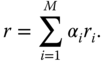
The question of a virtual multiple-input multiple-output (VMIMO) channel is especially vital in the case of cooperative relaying, where the notion of a fixed MEA is translated into a dynamic set of relay nodes forming a virtual antenna array (VAA) to exercise the operation of distributed space-time block coding. Given the fact that such a virtual multiple-input multiple-output radio channel is formed by relay nodes,9 it may in general be perceived as sufficiently, if not entirely, uncorrelated, which, in general, translates into the applicability of the theoretical gains attainable by legacy systems employing the classic MIMO approach, as long as a sufficiently high level of synchronism is guaranteed. One should note, however, that before the emergence of systems capable of exploiting transmission diversity in the spatial domain, radio transmission was generally performed in the temporal and frequential domain, over single-input single-output (SISO) or single-input multiple-output (SIMO) channels, as outlined in Figure 3.4. Then, once it turned out that additional information may, easily and efficiently, be conveyed over the third, spatial, dimension, the global scientific trends in this respect were immediately shifted towards multiple-input single-output (MISO) and MIMO-based technologies, as presented in Figure 3.5. In fact, from the mathematical perspective, the wireless multiple-input multiple-output10 radio channel in question is usually defined by a channel matrix (CM), denoted by ![]() , where the coefficients
, where the coefficients ![]() indicate the gains of the radio links formed between each transmitting antenna
indicate the gains of the radio links formed between each transmitting antenna ![]() (
(![]() ) and each receiving antenna
) and each receiving antenna ![]() (
(![]() ):
):
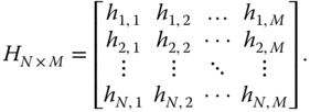

Figure 3.4 Single-input single-output and single-input multiple-output systems.

Figure 3.5 Multiple-input single-output and multiple-input multiple-output systems.
In order to fully quantify the potential behind such a channel representation, it suffices to make a comparison with the extraordinary milestone work of Shannon (1948), which, although it does not cover the most recent advancements in this respect, provides a thorough analysis of a SISO channel with additive white Gaussian noise (AWGN), for the sake of expressing a single user data rate bound, as described by the following formula, where ![]() represents the channel gain (CHG):
represents the channel gain (CHG):

The major strength of Equation 3.4 stems from the fact that it combines the channel capacity ![]() with the related channel bandwidth
with the related channel bandwidth ![]() and the SNR, expressed as the ratio of the transmitted signal power
and the SNR, expressed as the ratio of the transmitted signal power ![]() to the noise power
to the noise power ![]() . Fairly obviously, it would seem that the most straightforward method of increasing such a capacity, and, therefore, the attainable data rate bound, would consist in broadening the bandwidth of the radio channel (Wódczak, 2012a). Yet, setting aside technological considerations, given the fact that bandwidth is a commercially controlled product, such an approach would be too inefficient and costly, and consequently not justifiable. Going further, one could also potentially consider increasing the SNR; however, since such an approach would immediately translate into the need to increase the power of the transmitted signal, it would naturally enlarge the level of both the co-channel interference (CCI) and inter-channel interference (ICI). What is more, due to the logarithmic relation between both the parameters, the effectively attainable channel capacity gain (CCG) would be less significant when compared to the first case (Wódczak, 2012a).
. Fairly obviously, it would seem that the most straightforward method of increasing such a capacity, and, therefore, the attainable data rate bound, would consist in broadening the bandwidth of the radio channel (Wódczak, 2012a). Yet, setting aside technological considerations, given the fact that bandwidth is a commercially controlled product, such an approach would be too inefficient and costly, and consequently not justifiable. Going further, one could also potentially consider increasing the SNR; however, since such an approach would immediately translate into the need to increase the power of the transmitted signal, it would naturally enlarge the level of both the co-channel interference (CCI) and inter-channel interference (ICI). What is more, due to the logarithmic relation between both the parameters, the effectively attainable channel capacity gain (CCG) would be less significant when compared to the first case (Wódczak, 2012a).
As a result, there is no denying that the above issue would need to be resolved in some other way, and the situation changes immediately when MIMO11 technology is employed as outlined, for example, by Telatar (1999). In general, as long as the number of both the transmitting ![]() and receiving
and receiving ![]() antennae remains equal to 1, any throughput gain may amount merely to about 1 bit per Hz for each 3 dB increase in the SNR, as clearly explained by Foschini and Gans (1998). Should MEAs of size
antennae remains equal to 1, any throughput gain may amount merely to about 1 bit per Hz for each 3 dB increase in the SNR, as clearly explained by Foschini and Gans (1998). Should MEAs of size ![]() be employed at both ends of the radio channel, the achievable capacity would scale linearly with
be employed at both ends of the radio channel, the achievable capacity would scale linearly with ![]() , as proven by Lozano et al. (2001). Consequently, once again referring to the work of Foschini and Gans (1998), it appears feasible to achieve almost as many as
, as proven by Lozano et al. (2001). Consequently, once again referring to the work of Foschini and Gans (1998), it appears feasible to achieve almost as many as ![]() bits per Hz, and, in order to verify such a statement, one may follow, for example, Vucetic and Yuan (2003), where the singular-value decomposition (SVD) theorem is applied, according to which the previously introduced channel matrix
bits per Hz, and, in order to verify such a statement, one may follow, for example, Vucetic and Yuan (2003), where the singular-value decomposition (SVD) theorem is applied, according to which the previously introduced channel matrix ![]() (Equation 3.3) may be presented in the following rewritten form:
(Equation 3.3) may be presented in the following rewritten form:
In this case, ![]() is a nonnegative and diagonal matrix of size
is a nonnegative and diagonal matrix of size ![]() , while
, while ![]() and
and ![]() are unitary matrices of size
are unitary matrices of size ![]() and
and ![]() , respectively, where
, respectively, where ![]() denotes a Hermitian transposition. Clearly, the advantage of the SVD theorem lies in the fact that all the above-mentioned matrices are characterised by having nonzero elements solely on their main diagonals. What it implies mathematically is that
denotes a Hermitian transposition. Clearly, the advantage of the SVD theorem lies in the fact that all the above-mentioned matrices are characterised by having nonzero elements solely on their main diagonals. What it implies mathematically is that ![]() and
and ![]() , where
, where ![]() is the identity matrix of size
is the identity matrix of size ![]() , and
, and ![]() the identity matrix of size
the identity matrix of size ![]() (Vucetic and Yuan, 2003).
(Vucetic and Yuan, 2003).
Similarly, the diagonal entries of ![]() are equal to the nonnegative square roots of the eigenvalues of the matrix
are equal to the nonnegative square roots of the eigenvalues of the matrix ![]() and are denoted by
and are denoted by ![]() :
:
where ![]() is an eigenvector of size
is an eigenvector of size ![]() associated with
associated with ![]() . Based on the above, one might conclude most correctly that it is possible to think of an equivalent virtual multiple-input multiple-output (EVMIMO) channel comprising solely
. Based on the above, one might conclude most correctly that it is possible to think of an equivalent virtual multiple-input multiple-output (EVMIMO) channel comprising solely ![]() uncoupled parallel subchannels, with
uncoupled parallel subchannels, with ![]() being understood as the rank of the channel matrix
being understood as the rank of the channel matrix ![]() , and, thereby, presumably equal to at most the minimum of
, and, thereby, presumably equal to at most the minimum of ![]() and
and ![]() . This situation is outlined in Figure 3.6, where the concept of generic transmitters (GTs) and generic receivers (GRs) is presented, as originally introduced by Wódczak (2014).12 The generic transmitters and generic receivers will be denoted by
. This situation is outlined in Figure 3.6, where the concept of generic transmitters (GTs) and generic receivers (GRs) is presented, as originally introduced by Wódczak (2014).12 The generic transmitters and generic receivers will be denoted by ![]() and
and ![]() , respectively, where
, respectively, where ![]() and
and ![]() , or
, or ![]() and
and ![]() , depending on whether
, depending on whether ![]() or
or ![]() . Most generally, the said generic transmitters and generic receivers could be assumed to either take the form of the legacy MEA, or, as in the analysed case, to reflect the networked design, become perceived as relay nodes. Should the latter be the case, certain clarification might be necessary to avoid any unintended inconsistency, possibly resulting from the fact that MEAs are also covered. In other words, should the said relay nodes be homogeneous, and thus equipped with the same number of antennae, then
. Most generally, the said generic transmitters and generic receivers could be assumed to either take the form of the legacy MEA, or, as in the analysed case, to reflect the networked design, become perceived as relay nodes. Should the latter be the case, certain clarification might be necessary to avoid any unintended inconsistency, possibly resulting from the fact that MEAs are also covered. In other words, should the said relay nodes be homogeneous, and thus equipped with the same number of antennae, then ![]() would always be greater than
would always be greater than ![]() , as long as a virtual antenna array became instantiated.13
, as long as a virtual antenna array became instantiated.13

Figure 3.6 EVMIMO channel. Adapted from Vucetic and Yuan (2003).
3.2.3 Capacity, Modelling, and Gains
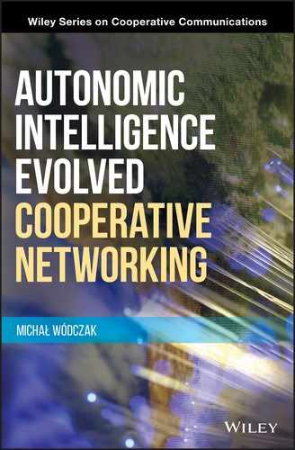
Attempting to visualise the attainable capacity of the equivalent virtual multiple-input multiple-output radio channel and following the example of Vucetic and Yuan (2003), yet assuming the most representative case where ![]() , so that the linear relation between the channel capacity and the number of generic transmitters or generic receivers could be emphasised, one could express the formula of channel capacity as follows, given that the det() function provides the determinant of a matrix:
, so that the linear relation between the channel capacity and the number of generic transmitters or generic receivers could be emphasised, one could express the formula of channel capacity as follows, given that the det() function provides the determinant of a matrix:

Here, ![]() would take the value of either
would take the value of either ![]() , for
, for ![]() , or
, or ![]() , for
, for ![]() . Bearing in mind that the generic transmitters and generic receivers would be virtually interconnected exclusively over the aforementioned orthogonal parallel subchannels, the respective channel matrix
. Bearing in mind that the generic transmitters and generic receivers would be virtually interconnected exclusively over the aforementioned orthogonal parallel subchannels, the respective channel matrix ![]() could be expressed as:
could be expressed as:
where ![]() denotes a scaling factor related to power normalisation, so that, following Vucetic and Yuan (2003), the capacity
denotes a scaling factor related to power normalisation, so that, following Vucetic and Yuan (2003), the capacity ![]() of the equivalent virtual multiple-input multiple-output radio channel could be rewritten as
of the equivalent virtual multiple-input multiple-output radio channel could be rewritten as

which, thanks to the existence of the unitary matrix ![]() in both the components of the logarithmic function, allowing for a direct translation into a diagonal matrix with the relevant expression on its main diagonal, may be rewritten, using diag() function to represent the diagonal matrix, as
in both the components of the logarithmic function, allowing for a direct translation into a diagonal matrix with the relevant expression on its main diagonal, may be rewritten, using diag() function to represent the diagonal matrix, as

Based on the properties of the determinant of such a matrix, which is equal to the product of the elements on its main diagonal, as well as applying basic logarithmic operations, one may further rewrite the equation in the form

Given the above, it immediately becomes clear that the capacity of the equivalent virtual multiple-input multiple-output radio channel may scale linearly with the number of generic transmitters or generic receivers. In fact, the normalised form of the achievable channel capacity is illustrated in Figure 3.7, where an equal number ![]() , ranging from 1 to 8, of generic transmitters and generic receivers is assumed. In general, such a potential may appear exploitable in two somewhat disjoint yet overlapping areas, following Molisch and Win (2004). Namely, on the one hand it is possible to create a highly effective diversity scheme to increase the robustness of the system against impairments induced by the radio channel, while on the other hand there is the option of transmitting multiple data streams in parallel to increase the system throughput (Wódczak, 2012a). Essentially, it all boils down to the characteristics of the underlying radio channel and, therefore, a properly adjusted mathematical model is required. For this reason, the approach to modelling cited below, as originally proposed by Zheng and Xiao (2003), is brought into the global picture of this book after having been thoroughly verified, in particular because it will be referred to for illustrative simulation purposes related to parts of the overall Autonomic Cooperative Networking Architectural Model. Thus, mutually comparable results are expected to be provided, which, given the complexity of the simulated components, may highly capitalise on the moderate computational complexity of this model.
, ranging from 1 to 8, of generic transmitters and generic receivers is assumed. In general, such a potential may appear exploitable in two somewhat disjoint yet overlapping areas, following Molisch and Win (2004). Namely, on the one hand it is possible to create a highly effective diversity scheme to increase the robustness of the system against impairments induced by the radio channel, while on the other hand there is the option of transmitting multiple data streams in parallel to increase the system throughput (Wódczak, 2012a). Essentially, it all boils down to the characteristics of the underlying radio channel and, therefore, a properly adjusted mathematical model is required. For this reason, the approach to modelling cited below, as originally proposed by Zheng and Xiao (2003), is brought into the global picture of this book after having been thoroughly verified, in particular because it will be referred to for illustrative simulation purposes related to parts of the overall Autonomic Cooperative Networking Architectural Model. Thus, mutually comparable results are expected to be provided, which, given the complexity of the simulated components, may highly capitalise on the moderate computational complexity of this model.

Figure 3.7 Capacity of VMIMO channel for  .
.
In particular, the model proposed by Zheng and Xiao (2003) has been chosen since it may be directly used for generating multiple uncorrelated fading waveforms for frequency-selective fading channels and diversity-combining scenarios, and especially for multiple-input multiple-output radio channels. As such, the model is capable of producing radio channel coefficients fully satisfying the reference Rayleigh distribution through the application of an elegantly straightforward sum-of-sinusoids statistical approach (Zheng and Xiao, 2003). The major advantage of the model in question stems from the fact that the autocorrelation and cross-correlation functions of the quadrature components, as well as the autocorrelation function of the complex envelope, all match the desired reference ones even when the number of sinusoids is expressed as a single digit number. As verified by the author, it suffices to use as few as five sinusoids to obtain a virtually ideal distribution. In particular, following Zheng and Xiao (2003), the normalised fading process of such a statistical model may be written as
where ![]() is defined by
is defined by

and ![]() is defined by
is defined by

while ![]() is
is
and the random variables ![]() ,
, ![]() , and
, and ![]() are all statistically independent and uniformly distributed over the range
are all statistically independent and uniformly distributed over the range ![]() for all values of
for all values of ![]() . The respective probability density function (PDF) for the apparently optimum number of five sinusoids is presented in Figure 3.8, to confirm the convergence efficiency.14
. The respective probability density function (PDF) for the apparently optimum number of five sinusoids is presented in Figure 3.8, to confirm the convergence efficiency.14

Figure 3.8 Probability density function for five sinusoids.
Last, but not least, keeping in mind the diversity-rooted origins of spatio-temporal processing and the general characteristics of the multiple-input multiple-output radio channel, it becomes necessary to introduce the notion of diversity gain (DG). In fact, diversity techniques are, in general, useful in terms of alleviating the impairments introduced by wireless communications translating themselves into signal quality deterioration related to the fading effect. As discussed by Jankiraman (2004), the larger the number of independent fading branches or paths, or simply the receiving antennae, the bigger the so-called diversity order (DO). Moving forward, following Larsson and Stoica (2003b), for example, one should note that once maximum likelihood detection (MLD) or maximal ratio combining is assumed, the average error probability in a region of high SNR values may be expressed as
where ![]() denotes the coding gain, according to Larsson and Stoica (2003b) also referred to as coding advantage (CA), which is provided by a block or convolutional coding scheme in the temporal domain, whereas
denotes the coding gain, according to Larsson and Stoica (2003b) also referred to as coding advantage (CA), which is provided by a block or convolutional coding scheme in the temporal domain, whereas ![]() represents directly the aforementioned diversity order. In particular, should the
represents directly the aforementioned diversity order. In particular, should the ![]() curve be plotted as a function of SNR on a log–log scale, then
curve be plotted as a function of SNR on a log–log scale, then ![]() would determine the horizontal position of this curve while
would determine the horizontal position of this curve while ![]() would correspond to its slope (Molisch and Win, 2004). What is more, thanks to the diversity order, the said diversity gain would be observable; it is defined as the gain provided by the spatial diversity across channels on the transmitter side, the receiver side, or both, allowing compensation for the fading effect (Jankiraman, 2004).
would correspond to its slope (Molisch and Win, 2004). What is more, thanks to the diversity order, the said diversity gain would be observable; it is defined as the gain provided by the spatial diversity across channels on the transmitter side, the receiver side, or both, allowing compensation for the fading effect (Jankiraman, 2004).
3.3 Space-Time Coding Techniques
3.3.1 Orthogonal Block-Coded Designs
Given the background established thus far with the introduction of the transmission medium in the form of the equivalent virtual multiple-input multiple-output radio channel along with all the related commentary on diversity, virtualisation, capacity, modelling, and gains, the time has come for the next step in advancing the analysis by shifting the focus onto the approach known as space-time block coding (STBC). In fact, not without sound justification was its extended version, distributed space-time block coding (DSTBC), highlighted in the opening chapter under the umbrella of spatio-temporal processing as one of the major technological pillars of the entire Autonomic Cooperative Networking Architectural Model. Regardless of its pivotal role to the entire design, one of the key advantages of space-time block coding consists in the fact that, as indicated by Jankiraman (2004), no channel state information (CSI) is required on the side of the transmitter, which, along with its orthogonality-driven design as proposed by Alamouti (1998), makes it one of the biggest technological advancements in the realm of modern wireless communications. In fact, looking at Figure 3.9, one may easily discern that such an STBC-enabled system shall perfectly match the previously discussed characteristics of the multiple-input multiple-output channel, as it is intended to exploit a transmitting MEA of size N and a receiving MEA of size M. In this context, the workings of space-time block coding are outlined below, along with example code matrices of further interest.

Figure 3.9 Diagram of space-time coded system.
In general, among other spatio-temporal processing techniques of potential relevance, which could be successfully employed for the pre-processing of the signals to be transmitted in such a way that they would become more robust to the impairments typically induced by the radio channel, there is the said space-time block coding; it is characterised (Alamouti, 1998) by the ability to offer the said diversity gain, yet it cannot offer any inherent option of introducing additional coding gain. Despite this, the value of space-time block coding should never be diminished, especially if outer coding is employed. What appears to be most interesting, however, is that, despite its commonly accepted name, in general the concept of space-time block coding should rather be perceived as a modulation and not an explicit coding technique. This is so, as the rationale behind its design was specifically directed towards the provision of additional diversity in both the spatial and temporal domains, should a wireless communications system employ MEAs with the objective of increasing its transmission capabilities. One should note, however, that the notion of MEAs is brought up solely for consistency reasons and, as was the case for the multiple-input multiple-output radio channel eventually being upgraded to its counterpart in the form of the equivalent virtual multiple-input multiple-output radio channel, MEAs are immediately replaced with generic transmitters and generic receivers, as outlined in Figure 3.10, in order to pave the way for the ultimate transition from space-time block coding into its networked concept of distributed space-time block coding.

Figure 3.10 Generic space-time coded  system. Adapted from Alamouti (1998).
However, apart from all the advantages of space-time block coding signalled thus far, no sooner does the major selling point behind this technology become clear than the comparison with legacy approaches to reception diversity is made. It then immediately transpires that space-time block coding allows for the complexity related to the deployment of multiple antennae on small mobile UTs to be shifted to a BS or an AP. Such an approach is highly advantageous because the complexity of the UTs can be reduced, and the cost of installing a single MEA solely on the BS or AP side appears less substantial, while the spacing among the elements of such an MEA may no longer be physically limited. As much as this capability could be appealing when more classic use cases are concerned, the above-mentioned argument may no longer remain fully convincing should the ultimate distributed space-time block coding be taken into account, especially because, in such a case, those will be the relay nodes to become preselected to form a virtual antenna array expected to behave in a way resembling a dynamic MEA. One should note, however, that a use case of this type already seems to go well beyond the assumptions inherent in the classic version of STBC, where MEAs would normally be employed. The technological upgrade results from the fact that the approach to the design of the Autonomic Cooperative Networking Architectural Model fairly frequently induces certain changes to legacy operation of the leveraged technologies.
In order to discuss the manner in which transmission based on a complex orthogonal design15 may operate, the initial version of such an approach is first introduced as invented by Alamouti (1998), who defined it using the ![]() code matrix (3.17). While its operation follows the precise pattern of two consecutive time slots, the
code matrix (3.17). While its operation follows the precise pattern of two consecutive time slots, the ![]() code was designed for a system employing strictly two generic transmitters and an unlimited number of generic receivers. In particular, moving into its workings, and following the pattern of the
code was designed for a system employing strictly two generic transmitters and an unlimited number of generic receivers. In particular, moving into its workings, and following the pattern of the ![]() matrix, during the first time slot both the
matrix, during the first time slot both the ![]() and
and ![]() symbols are transmitted by the first and second generic transmitters, respectively, while during the second time slot both the
symbols are transmitted by the first and second generic transmitters, respectively, while during the second time slot both the ![]() and
and ![]() symbols are transmitted in exactly the same manner by the same generic transmitters.
symbols are transmitted in exactly the same manner by the same generic transmitters.

One should note, however, that there exist more complicated space-time block coding matrices, just to mention the generalised complex orthogonal designs (GCODs), which were additionally and separately invented and proposed by Tarokh et al., 1999a,b. Such enhanced designs include the ![]() (Equation 3.18),
(Equation 3.18), ![]() (Equation 3.19),
(Equation 3.19), ![]() (Equation 3.20), and
(Equation 3.20), and ![]() (Equation 3.21) code matrices, which are applicable when sets of generic transmitters larger than two are to be employed. What is more, it is also necessary to keep in mind that there is a trade-off between the robustness of these codes and their code rates (CDRs) being strictly related to the number of generic transmitters. In fact, the code rate is equal to 1 only in the case of the
(Equation 3.21) code matrices, which are applicable when sets of generic transmitters larger than two are to be employed. What is more, it is also necessary to keep in mind that there is a trade-off between the robustness of these codes and their code rates (CDRs) being strictly related to the number of generic transmitters. In fact, the code rate is equal to 1 only in the case of the ![]() code; although more reliable, the other codes offer worse code rates, equal to
code; although more reliable, the other codes offer worse code rates, equal to ![]() for the
for the ![]() and
and ![]() matrices and
matrices and ![]() for
for ![]() and
and ![]() .
.


Moreover, with the passage of time there have been many approaches to space-time block coding proposed in pursuit of achieving the often disjoint, at least when generalised complex orthogonal designs are concerned, objectives of increasing the number of generic transmitters and the related code rate at the same time. In particular, attempting to complement the above classic code matrices by analysing the further milestone developments in this area, one may, in the first place, come across the work of Su and Xia (2003), where a couple of generalised complex orthogonal designs capable of using five and six generic transmitters and characterised by code rates of ![]() and
and ![]() , respectively, were proposed. Then, a full-rate GCOD was proposed by Jewel and Rahman (2009) which could employ four generic transmitters, and this was complemented by another full-rate GCOD proposed by Murthya and Gowrib (2012) which, in turn, could accommodate as many as eight generic transmitters. Interesting though it may seem, should the criterion of orthogonality be relaxed even slightly, one may not only discover quasi-orthogonal (QO) full-rate and full-diversity designs proposed by Jung et al. (2008) and capable of employing any odd number of generic transmitters, but many other concepts of relevance displaying novelty with regard to different aspects of spatio-temporal processing. However, any further classification of these is beyond the scope of this book; the above-mentioned code matrices will be referred to at a later stage.
, respectively, were proposed. Then, a full-rate GCOD was proposed by Jewel and Rahman (2009) which could employ four generic transmitters, and this was complemented by another full-rate GCOD proposed by Murthya and Gowrib (2012) which, in turn, could accommodate as many as eight generic transmitters. Interesting though it may seem, should the criterion of orthogonality be relaxed even slightly, one may not only discover quasi-orthogonal (QO) full-rate and full-diversity designs proposed by Jung et al. (2008) and capable of employing any odd number of generic transmitters, but many other concepts of relevance displaying novelty with regard to different aspects of spatio-temporal processing. However, any further classification of these is beyond the scope of this book; the above-mentioned code matrices will be referred to at a later stage.
3.3.2 Derivation of Decoding Metrics
Even though, as it has already been highlighted, there apparently exist a variety of relevant spatio-temporal processing techniques, fairly thoroughly scrutinised in the literature, the focus from now on in this book will be deliberately limited to space-time block coding. Such an assumption is being made despite the fact that one could contemplate using any other relevant approach to spatio-temporal processing as a replacement. Given the objective and theme of this book, such a replacement should not be expected to incur any substantial changes to the most crucial architectural assumptions governing the place and role of the major components of the presented system design. In this respect, more precisely, the code matrices presented thus far, which fulfil the generalised complex orthogonal design criterion to be outlined in detail below, will be employed for further analyses related to the comprehensive depiction of the workings of the Autonomic Cooperative Networking Architectural Model. Given such an approach, it is necessary to provide a high-level overview of the decoding process, mostly for quick reference reasons. However, in scrutinising the literature covering the topic of space-time block coding the author gained the impression that there may exist some inconsistency in the mathematical forms of the decoding metrics, manifested in certain apparently unintentional typographical errors. In order to resolve any doubts potentially arising from the above observation, all the pertinent metrics been recalculated by the author, and they are presented with a commentary intended to indicate the said inconsistencies, when applicable.
In particular, moving to the reception side of the system, it might be the case that a generic receiver is equipped with an MEA to obtain an even better performance. Should this be the case, the radio signal received by receiving antenna ![]() could be expressed as (Alamouti, 1998)
could be expressed as (Alamouti, 1998)

where ![]() denotes the channel coefficient previously defined for the multiple-input multiple-output channel matrix (Equation 3.3),
denotes the channel coefficient previously defined for the multiple-input multiple-output channel matrix (Equation 3.3), ![]() represents the symbol transmitted by the antenna of the generic transmitter16
represents the symbol transmitted by the antenna of the generic transmitter16 ![]() , and the noise samples
, and the noise samples ![]() are modelled by a complex Gaussian process of zero mean and
are modelled by a complex Gaussian process of zero mean and ![]() variance per dimension. This is, in fact, where the condition of GCOD comes into the global picture of space-time block coding, being the main condition under which the operation of decoding may be successfully performed. Following the work of Larsson and Stoica (2003a), for example, the condition of orthogonality may be defined as
variance per dimension. This is, in fact, where the condition of GCOD comes into the global picture of space-time block coding, being the main condition under which the operation of decoding may be successfully performed. Following the work of Larsson and Stoica (2003a), for example, the condition of orthogonality may be defined as

where ![]() is the number of generic transmitters and
is the number of generic transmitters and ![]() is the
is the ![]() identity matrix. The process of decoding is based on MLD, aiming to minimise the decision metric as defined by Tarokh et al. (1999a):
identity matrix. The process of decoding is based on MLD, aiming to minimise the decision metric as defined by Tarokh et al. (1999a):

This metric can easily be derived on the basis of the theory outlined, for instance, by Goldsmith (2005). In order to account for such a mathematical formula, one should note that its most obvious interpretation boils down to the fact that, for a given code, those potentially transmitted symbols are chosen which minimise this metric. Unfortunately, its use in the above form would render the calculation process computationally inefficient.
Therefore, to address this issue, a set of relevantly modified metrics was introduced by Tarokh et al. (1999b). In particular, for the ![]() code matrix (Equation 3.17), the metric in Equation 3.24 may be rewritten as
code matrix (Equation 3.17), the metric in Equation 3.24 may be rewritten as

While MLD aims to find the minimum value of this metric for all possible combinations of the variables ![]() and
and ![]() , given the attempt at avoiding the aforementioned computational inefficiency, the above expression may be expanded so that the terms independent of the said variables can be deleted. In other words, the problem of the minimisation of this metric becomes equivalent to minimising the following expression:
, given the attempt at avoiding the aforementioned computational inefficiency, the above expression may be expanded so that the terms independent of the said variables can be deleted. In other words, the problem of the minimisation of this metric becomes equivalent to minimising the following expression:
Such a formula, in turn, may be clearly perceived as being composed of two components, the former being exclusively a function of the variable ![]() , while the latter being exclusively a function of the variable
, while the latter being exclusively a function of the variable ![]() . As a result, one may conclude that the total value of this metric is a minimum when each of these components is a minimum. Consequently, following Tarokh et al. (1999b), the metric for the
. As a result, one may conclude that the total value of this metric is a minimum when each of these components is a minimum. Consequently, following Tarokh et al. (1999b), the metric for the ![]() code can be expressed as
code can be expressed as

where for ![]() the signal
the signal ![]() received by antenna
received by antenna ![]() is given by
is given by
and for ![]() the signal
the signal ![]() received by antenna
received by antenna ![]() is given by
is given by
Similarly, the metric for the ![]() code may be written as
code may be written as

where for ![]() the signal
the signal ![]() received by antenna
received by antenna ![]() is given by
is given by
for ![]() the signal
the signal ![]() received by antenna
received by antenna ![]() is given by
is given by
for ![]() the signal
the signal ![]() received by antenna
received by antenna ![]() is given by
is given by
and for ![]() the signal
the signal ![]() received by antenna
received by antenna ![]() is given by
is given by
Similarly again, the metric for the ![]() code can be expressed as
code can be expressed as
where for ![]() the signal
the signal ![]() received by antenna
received by antenna ![]() is given by
is given by
for ![]() the signal
the signal ![]() received by antenna
received by antenna ![]() is given by
is given by
for ![]() the signal
the signal ![]() received by antenna
received by antenna ![]() is given by
is given by
and for ![]() the signal
the signal ![]() received by antenna
received by antenna ![]() is given by17
is given by17
The metric for the ![]() code can similarly be written as
code can similarly be written as

where for ![]() the signal
the signal ![]() received by antenna
received by antenna ![]() is given by
is given by

for ![]() the signal
the signal ![]() received by antenna
received by antenna ![]() is given by
is given by

and for ![]() the signal
the signal ![]() received by antenna
received by antenna ![]() is given by
is given by

Finally, the metric for the ![]() code can be written as
code can be written as

where for ![]() the signal
the signal ![]() received by antenna
received by antenna ![]() is given by
is given by

for ![]() the signal
the signal ![]() received by antenna
received by antenna ![]() is given by
is given by

and for ![]() the signal
the signal ![]() received by antenna
received by antenna ![]() is given by
is given by

3.3.3 Trellis-Coded Approach
In the quest for further improvement, two different paths were followed, the first of them, to be yet revisited, in the form of a trellis coded modulation (TCM) driven, concatenated version of space-time block coding, as proposed by Alamouti et al. (1998), and, the second one, assuming an all-in-one solution of space-time trellis coding (STTC), as introduced in the publications of Tarokh et al. (1998, 1999c). Commencing the analysis with the latter approach, when compared to space-time block coding, mostly perceived as a modulation technique, space-time trellis coding intends to capitalise on additional relations not only between specific sequences transmitted by distinct Generic Transmitters, but also between the symbols being the constituents of such sequences, so that apart from the discussed diversity gain, additional coding gain may be observed, too. Most naturally, the trellis-coded nature of this approach should be perceived as being inherently embedded into the structure of the space-time-driven arrangement itself. Quite the opposite occurs when the former concatenated solution is considered: despite a certain level of integration, especially on the side of the very outer TCM, the underlying inner space-time block coding still seems, undeniably, detachable. Even though the level of internal integration clearly differs between the two trellis-coded approaches, the former will be especially emphasised once the latter has been outlined in more detail, chiefly because, as additionally elaborated by Gong and Letaief (2002), this type of concatenation may prove to outperform even an STTC-based design, making it especially interesting given the major theme of this book.

Figure 3.11 Base code for 4-PSK modulation. Adapted from Tarokh et al. (1998).
Following Tarokh et al. (1998), the base code trellis exploiting the phase-shift keying (PSK) modulation, in the form of 4-PSK, is presented in Figure 3.11. Examining the structure of such a code, one should note that the order of the numbers placed to the left of the corresponding trellis diagram should be interpreted in a specific way: the most significant digit represents the information on the current state, while the least significant one corresponds not only to the input itself, but particularly to the next state, to which the transition is to be made. In other words, consecutive pairs of bits arriving at the input of the respective encoder would determine the transition from the current state to the following one, where two symbols would be relayed to the generic transmitters in such a way that the first generic transmitter would transmit the channel symbol informing about the current state, while the second generic transmitter would transmit the channel symbol corresponding to the next state. The process of decoding, in turn, is based on the widely recognised algorithm by Viterbi (1967), the logic of which revolves around the fact that each transition on the trellis diagram is assigned a metric value, in this case calculated according to the formula devised by Tarokh et al. (1998):

where ![]() and
and ![]() denote the consecutive trellis states between which a given transition is taking place. Assuming no channel impairments, the decoding procedure of an example input sequence of
denote the consecutive trellis states between which a given transition is taking place. Assuming no channel impairments, the decoding procedure of an example input sequence of ![]() fed to the space-time code trellis illustrated in Figure 3.11 would be carried out in accordance with Figure 3.12 (Wódczak, 2012a).
fed to the space-time code trellis illustrated in Figure 3.11 would be carried out in accordance with Figure 3.12 (Wódczak, 2012a).

Figure 3.12 Example of STTC decoding process.
In particular, assume the encoder is initially in the zero state, and at each moment ![]() it can transition from the current state to the next one in the subsequent moment
it can transition from the current state to the next one in the subsequent moment ![]() , given one of the input values of
, given one of the input values of ![]() . Thus, the input sequence could be translated into the passage of the symbol pairs
. Thus, the input sequence could be translated into the passage of the symbol pairs ![]() to the generic transmitters. In such a context, keeping in mind the assumed nomenclature, the first generic transmitter would transmit the signals corresponding to the symbol sequence
to the generic transmitters. In such a context, keeping in mind the assumed nomenclature, the first generic transmitter would transmit the signals corresponding to the symbol sequence ![]() , while, concurrently, the second generic transmitter would transmit the signals corresponding to the symbol sequence
, while, concurrently, the second generic transmitter would transmit the signals corresponding to the symbol sequence ![]() . More precisely, this would mean that the respective modulated sequences of
. More precisely, this would mean that the respective modulated sequences of ![]() and
and ![]() would be observed at the output of the modulator. In other words, during the first modulation interval the
would be observed at the output of the modulator. In other words, during the first modulation interval the ![]() signal pair,
signal pair, ![]() , would be transmitted, so that, referring to Equation 3.22, the received signal could be written as
, would be transmitted, so that, referring to Equation 3.22, the received signal could be written as ![]() . Consequently, according to Equation 3.48, the following metrics would be calculated for their corresponding transitions:
. Consequently, according to Equation 3.48, the following metrics would be calculated for their corresponding transitions: ![]() ,
, ![]() ,
, ![]() ,
, ![]() . Then, the same procedure would be performed during the second modulation interval, where the signal pair
. Then, the same procedure would be performed during the second modulation interval, where the signal pair ![]() would be transmitted. The received signal could be expressed as
would be transmitted. The received signal could be expressed as ![]() , while the metrics would take the values of:
, while the metrics would take the values of: ![]() ,
, ![]() ,
, ![]() ,
, ![]() ,
, ![]() ,
, ![]() ,
, ![]() ,
, ![]() ,
, ![]() ,
, ![]() ,
, ![]() ,
, ![]() ,
, ![]() ,
, ![]() ,
, ![]() ,
, ![]() . As this process continues, a number of possible paths could lead to the same trellis state.
. As this process continues, a number of possible paths could lead to the same trellis state.
Essentially, given the rationale behind the aforementioned Viterbi algorithm, should more than one path cross the same trellis state at a given modulation interval, proceeding according to a certain rule referred to below, the path characterised by the lowest cumulative metric would need to be chosen. Looking at the illustrative example above, one may discern that apparently there would be as many as four candidate paths to be taken into account, and, if the selection decision were to be taken at this (normally too early) stage, then it would be the path in bold in Figure 3.12 that would be selected. However, one should note immediately that usually the analysis of such a trellis diagram should proceed as far as from three to five times the constraint length of the convolutional code for the sake of guaranteeing that the most reliable decisions are taken (Wesołowski, 2002). Given the related performance results depicted in Figure 3.13, there also exist more advanced codes in this respect, for example those proposed by Tarokh et al. (1998) and shown in Figures 3.14 and 3.15. While both these code trellis graphs are based on the same number of eight states and are generally designed for the PSK modulation scheme, the former follows the 4-PSK constellation pattern, while the latter reflects the application of the 8-PSK one. In this context, the focus is now going to shift slightly from space-time trellis coding in order to touch upon the alternative approach consisting in the employment of a TCM-driven, concatenated version of space-time block coding, where the additional operation of interleaving is exploited for better performance, as outlined, for example, by Gong and Letaief (2002).

Figure 3.13 Performance of STTC in AWGN channel.

Figure 3.14 Example of STTC with 4-PSK modulation. Adapted from Tarokh et al. (1998).

Figure 3.15 Example of STTC with 8-PSK modulation. Adapted from Tarokh et al. (1998).
As such, on the transmitting side the system exploits a TCM encoder responsible for the generation of a sequence of complex symbols, the consecutive vector of which, once interleaved, is submitted to the space-time block encoder (STBE) to perform, in the previously explained manner, the rather modulation-related operation outlined in Figure 3.16. Where the receiving side is concerned, the entire chain of processing modules is generally reversed by first involving the space-time block decoder (STBD) so that its output sequence, after having been deinterleaved, may be submitted to the TCM decoder, where the familiar operation of Viterbi decoding takes place, as indicated by Gong and Letaief (2002). Apparently, in order to be able to really capitalise on such a communication setup, one would need to establish a set of relevant criteria defining the proper construction of appropriate trellis codes, so that it could operate under the assumption of a specific fading process conditioned by the characteristics of the radio channel (Gong and Letaief, 2002). Should the reader be interested in additional details, the cited material is suggested as further reference since, despite the unquestionable advantages of the summarised trellis-based approaches, the major focus in this book will remain on space-time block coding, to be additionally advanced with the introduction of the equivalent distributed space-time block encoder (EDSTBE) as the plot unfolds more towards networked designs relating to cooperative relaying, after special emphasis has been placed on the protocol level architectural extensions.

Figure 3.16 Concatenated STBC with TCM. Adapted from Gong and Letaief (2002).
3.4 Protocol Level Overlay Logic
3.4.1 Autonomic Cooperative Node
Given the initial overview of the high-level incarnation of the Autonomic Cooperative Networking Architectural Model in the opening chapter and the analysis of the relevant spatio-temporal processing techniques introduced in this chapter, the time has come to commence the incremental and detailed presentation of the proposed architectural design in a bottom-up manner, beginning with the workings of both the vertically orientated physical layer, inherent in the Open Systems Interconnection Reference Model, and the horizontally positioned protocol level, embedded in the Generic Autonomic Network Architecture. In fact, once the description has been advanced, it will immediately become more than apparent that the already implied lack of correspondence between the layers and levels is highly factual, causing the conceptual overhead required to maintain consistency between the incrementally expanding design stages. In particular, the Autonomic Cooperative Node (ACN), to be scrutinised in more detail below, appears to serve as a highly representative example of such a situation, simply because it extends way beyond the protocol level. Consequently, it has been assumed by the author that whenever a fairly monolithic concept is to be referred to, its entire architectural structure will be presented in a general form at the introductory stage, even though some of its parts may not yet seem directly relevant. Thus, once the relation between autonomics and cooperation has been described, the concept of an Autonomic Cooperative Node will be outlined in the above-mentioned manner so that it may be complemented with the adopted interaction model over the protocol stack.
In the light of the above introduction, chiefly for the sake of reflecting the necessity of paving the ground for further developments, yet still before the rationale behind the Autonomic Cooperative Node may be introduced, the question of mutual relation between autonomics and cooperation is to be addressed, assuming certain dose of abstraction. On the one hand, the inherent feature of biologically inspired autonomics may be directly translated into the capacity of such a networked system to perform self-management through the orchestration of its behaviour, presumably without any configuration, optimisation, healing, or protection-related intervention from a network operator (Bicocchi and Zambonelli, 2007; Nakano, 2011). On the other hand, however, the, somewhat, similarly inherent, yet maybe a bit less exposed, idea of instantiating cooperation among the network nodes of such a system appears to imply that cooperation might add constructively to an increase of overall system resiliency in many different dimensions, as justified by Wódczak (2014). Keeping in mind the above context, where the whole networked system was termed autonomic, there is no reason why the concept of a cooperation-enabled node could not be integrated into the bigger picture of the same. Looking at the legacy autonomic node of the Generic Autonomic Network Architecture, however, the highly relevant question arises of how the flavour of being cooperative should be integrated into its logic, so that its self-managing nature could not be perceived as posing any preclusion in this respect.
Nonetheless, there is little wonder that, at least at first sight, should both the terms of autonomics and cooperation be subject to a joint treatment, they could be, somewhat, perceived as if they were stemming from two disjoint perspectives of being mutually exclusive. To be able to account for such a duality, one could consider two fairly contradictory connotations, especially should it be possible to imagine that a preselected set of cooperative network nodes might form a unified entity. On the one hand, this entity could be understood as an atomic embodiment of all those network nodes in the sense that there should not exist any contradiction between any two or more of its members. On the other hand, however, should the assumption of atomicity not fully hold, as might be the case in reality, the member network nodes could equally well express egoistic tendencies. Most obviously, such tendencies would not necessarily translate immediately into any intentional or deliberate actions, but, given the rationale behind the functioning of an autonomic system, they could be expected to rather result from a specific design, possibly not being able to handle all the potential behaviour stemming from dissociated policies, imposed either internally or externally. In general, such a connotation shall seem more inherent in artificial-intelligence-orientated approaches, where the system would be expected to reason and take, in some sense, ‘learned’ decisions by itself. Even though the notion of autonomic intelligence also assumes a certain flavour of cognition, it appears that the primary metaphor of the human autonomic nervous system should take precedence, thereby exposing the drive to achieve a commonly constructive state of global equilibrium.
As such, the instantiation of the Autonomic Cooperative Node, being one of the core functionalities of the entire Autonomic Cooperative Networking Architectural Model, definitely requires certain extensions to be proposed on top of the workings of the previously introduced elements of the Generic Autonomic Network Architecture. One such extension, Autonomic Cooperative Behaviour (ACB), becomes of special interest at this stage of the analysis because of its becoming directly responsible for enforcing the upgrade of the legacy autonomic node to the Autonomic Cooperative Node in question. In order to create a fully comprehensive context, however, one may need to go back to the foundations of the Generic Autonomic Network Architecture itself, where the ability to perform the key task of auto-discovery, possibly spanning multiple levels of abstraction, as only generally touched upon by Meriem et al. (2016), appears to be critically instrumental in incorporating the notion of cooperation into the global picture of autonomics. It is claimed to be so, since the performance of such a task is predominantly related to the possibility of answering the question of whether the target Autonomic Cooperative Node should operate in its fully-fledged and newly designed version, as it is yet to be outlined, or maybe it should fall back to, at least from the perspective of this book, the already outdated autonomic node related mode of operation due to backwards compatibility justified reasons.

Figure 3.17 ACNs from a level-driven orthogonal perspective.
Moving into the details, the proposed conceptual outline of an Autonomic Cooperative Node is depicted in Figure 3.17,18 where a set of comprehensively drafted and mutually aligned decision elements of relevance is presented.19 Not only should these decision elements be perceived as instrumental in the functioning of the entire Autonomic Cooperative Networking Architectural Model, but the existence and scope of the previously introduced levels of abstraction, inherent in the Generic Autonomic Network Architecture, should remain virtually unaltered (Wódczak, 2012a). In particular, perceiving the entire setup from the usually assumed bottom-up perspective, first comes the protocol level where the cooperative transmission decision element (CTDE) is deployed with the intention of combining the equivalent virtual multiple-input multiple-output radio channel inherent in the physical layer with the distributed space-time block coding belonging to the link layer, so that the above-mentioned ACSs may be created, where the instantiation of cooperative transmission is assumed to be taking place. Next, in the upward direction, is the cooperative re-routing decision element (CRDE) of the function level, responsible mainly for providing additional dependability. This is achieved through interaction with two other decision elements of relevance in the form of the interrelated resilience and survivability decision element (RSDE) and fault management decision element (FMDE), both being able to jointly identify the root causes and symptoms to infer that a physical or logical system failure may be imminent (Wódczak, 2014). Consequently, the pertinent cooperative re-routing procedure may be triggered well ahead of any accordingly foreseeable failure to ensure that overall service continuity is properly guaranteed.

Figure 3.18 Interaction over protocol stack.
Progressing further towards the node level, one may clearly discern expansion of complementary decision-making logic with special focus on the incorporation of the management of a cross-layer driven interaction between the said distributed space-time block coding of the link layer and the multi-point relay (MPR) station selection heuristics of the Optimised Link State Routing (OLSR) protocol residing at the network layer for the needs of guaranteeing that the Autonomic Cooperative Nodes of interest may become properly assigned to their most respective autonomic cooperative sets. Last, but not least, comes the top-most cooperation orchestration decision element (CODE) located at the network level, responsible for overseeing the ACB-related interactions under the umbrella of the Autonomic Cooperative Networking Architectural Model. Given the above context of the presented entities, one should keep in mind that such an overlay stemming from the Generic Autonomic Network Architecture should be perceived as perpendicular to the protocol stack based on the Open Systems Interconnection Reference Model. It is deemed to be so since the role of said overlay should consist in interacting with and steering various protocols of the pertinent stack, while communication between or among various Autonomic Cooperative Nodes would still need to follow the typical encapsulation process performed over that stack, as generally outlined in Figure 3.18, in the light of Wódczak (2012a).
Following the above assumptions, as well as taking into account the nature of wireless communications, should a given source node (SN) decide to transmit data packets towards a chosen destination node (DN), possibly located two hops away, such a transmission would most obviously be heard not only by the intermediate Autonomic Cooperative Nodes, presumably intending to instantiate Autonomic Cooperative Behaviour, but also by the other neighbours residing within the same range.20 To reduce protocol overhead, those Autonomic Cooperative Nodes not preselected to cooperate should silently discard any such received packets. The relevant operation would already be performed at the link layer, taking the responsibility of encoding and encapsulating the packets coming from the network layer into link layer frames, as well as performing proper physical addressing, thereby making communication with the specified one-hop neighbour or neighbours possible (Wódczak, 2014). Finally, each link layer frame would be encapsulated into a physical layer frame, and, after having been modulated, physically transmitted over the wireless medium. Consequently, the dynamic composition of Autonomic Cooperative Behaviour using the cross-layer-orientated Autonomic Cooperative Networking Protocol would be intended to minimise the probability of occurrence of any undesirable propagation effects, thereby making the process of communication efficient and uninterrupted, as indicated by Wódczak (2011b). Since the protocol stack would need to be implemented by every Autonomic Cooperative Node, the orchestration shall take place at the level of the overall Autonomic Cooperative System Architectural Model, respectively.
3.4.2 Cooperative Transmission Decision Element
Having established the detailed rationale behind the Autonomic Cooperative Node, according to which its management takes place at all the levels of abstraction belonging to the Generic Autonomic Network Architecture, it becomes natural to provide an incrementally developing insight into the specific levels. Given the generally followed bottom-up approach, the CTDE, residing in the lowest protocol level, is going to be examined in the present chapter with special emphasis on its internal logic, in the first order, leaving the architectural integration aspects for later consideration, scheduled to follow closely behind. Such a pattern will be repeated in the upcoming chapters so that, eventually, a comprehensively composed and fully-fledged instantiation of the Autonomic Cooperative Networking Architectural Model may be presented. Going back to the CTDE, however, before its internal logic can be outlined it is important to account for the differences in the semantics of the word ‘protocol’, not only when perceived from the internally disjoint perspectives of the layers of the Open Systems Interconnection Reference Model, but also keeping in mind one of the levels of the Generic Autonomic Network Architecture. Next, the internal logic will be explored through the workings of the equivalent virtual multiple input multiple output radio channel of the physical layer in the context of the distributed space-time block coding of the link layer, yet without any function level orchestration. Finally, certain performance-related conclusions will be drawn on the basis of the obtained simulation evaluation results (Wódczak, 2012a).
Looking at the semantics, one can see that the bottom-up approach may, somewhat unintentionally, appear to create a conceptual mismatch, especially given the fact that the CTDE of the protocol level is apparently bound to interact directly with the physical layer. To account for such a situation it is necessary to understand that, even though, on the protocol side, the pertinent functionality of the distributed space-time block coding belongs much more to the link layer, the previously explained modulation-driven nature of the general version of space-time block coding obviously calls for substantial involvement of the physical layer, too. What is more, however, there is also the question of the above-mentioned internally disjoint perspectives of the layers of the Open Systems Interconnection Reference Model itself, stemming from the difference between the notion of link layer and network layer protocols. In other words, while the distributed space-time block coding undoubtedly falls into what is most often categorised as cooperative relaying protocols, a much more prudent naming approach would rather involve the notion of a ‘scheme’, leaving ‘protocol’ where it should more naturally belong.21 As the above issues are considered deeply in the chapters to follow, it may transpire that the overall Autonomic Cooperative Networking Architectural Model will be strongly cross-layer driven, starting with ACSs, intended to bind both the physical layer and link layer, to arrive at the Autonomic Cooperative Networking Protocol, aiming to synergise both the link layer and network layer, yet to much higher an extent
The CTDE is assumed to be responsible for the orchestration of two-hop cooperative transmission on the path from the source node (SN), denoted as ![]() , towards the destination node (DN), denoted as
, towards the destination node (DN), denoted as ![]() , with the support of a set of Autonomic Cooperative Nodes, denoted as
, with the support of a set of Autonomic Cooperative Nodes, denoted as ![]() and located between them (Wódczak, 2014).22 In particular, a set of channel coefficients, denoted as
and located between them (Wódczak, 2014).22 In particular, a set of channel coefficients, denoted as ![]() , is maintained for all the radio links between the Autonomic Cooperative Nodes, conceptually belonging to the one-hop neighbourhood of
, is maintained for all the radio links between the Autonomic Cooperative Nodes, conceptually belonging to the one-hop neighbourhood of ![]() , and
, and ![]() , located in the two-hop neighbourhood of the same
, located in the two-hop neighbourhood of the same ![]() (Wódczak, 2012a). The parameters of these radio links are continually monitored within the hierarchical autonomic control loop pertinent to the CTDE, so that they may be verified against a preset threshold value, denoted as
(Wódczak, 2012a). The parameters of these radio links are continually monitored within the hierarchical autonomic control loop pertinent to the CTDE, so that they may be verified against a preset threshold value, denoted as ![]() . Consequently, and taking into account any policies imposed, the CTDE is responsible for the decision whether the cooperative transmission to take place over the equivalent virtual multiple-input multiple-output radio channel should be assisted by either three or four intermediary Autonomic Cooperative Nodes, acting according to either the
. Consequently, and taking into account any policies imposed, the CTDE is responsible for the decision whether the cooperative transmission to take place over the equivalent virtual multiple-input multiple-output radio channel should be assisted by either three or four intermediary Autonomic Cooperative Nodes, acting according to either the ![]() or
or ![]() code matrix. Other schemes could obviously also be applied, yet these two have been chosen to allow immediate comparison of the results, as each of them is characterised by the same code rate of
code matrix. Other schemes could obviously also be applied, yet these two have been chosen to allow immediate comparison of the results, as each of them is characterised by the same code rate of ![]() (Tarokh et al., 1999a). Clearly,
(Tarokh et al., 1999a). Clearly, ![]() constituted in this way should be perceived as a group of Autonomic Cooperative Nodes expressing Autonomic Cooperative Behaviour through the instantiation of the distributed space-time block coding (Wódczak, 2014).
constituted in this way should be perceived as a group of Autonomic Cooperative Nodes expressing Autonomic Cooperative Behaviour through the instantiation of the distributed space-time block coding (Wódczak, 2014).
The logic of the CTDE may be summarised as adapted in Algorithm 3.1.23 In particular, the ![]() mode becomes selected should the minimum value of the moduli contained in the
mode becomes selected should the minimum value of the moduli contained in the ![]() set turn out lower than the threshold
set turn out lower than the threshold ![]() (Wódczak, 2012a). As a result, one of the four allowable Autonomic Cooperative Nodes may no longer remain in the ACS, so that only the other three could still be involved in cooperative transmission. Otherwise, all four Autonomic Cooperative Nodes would be used, thereby making the distributed space-time block coding operate in
(Wódczak, 2012a). As a result, one of the four allowable Autonomic Cooperative Nodes may no longer remain in the ACS, so that only the other three could still be involved in cooperative transmission. Otherwise, all four Autonomic Cooperative Nodes would be used, thereby making the distributed space-time block coding operate in ![]() mode, as outlined by Wódczak (2011a). In this way, the worst radio link would be autonomically discarded until its parameters, monitored within the hierarchical autonomic control loop, once again meet the selection criterion of the logic behind the CTDE. However, one should also keep in mind that the monitoring data pertinent to such radio links may equally well be overridden by certain policies imposed by a higher-level decision element, such as the cooperation management decision element to be yet analysed. Should this happen, this type of situation would be the most representative manifestation of the cross-layer nature of the entire Autonomic Cooperative Networking Architectural Model, as the above link layer could become notified by the network layer that, for example, for quality of service reasons, it would be better to move one of the Autonomic Cooperative Nodes to another ACS, of which there may be many, to increase the overall routing efficiency.
mode, as outlined by Wódczak (2011a). In this way, the worst radio link would be autonomically discarded until its parameters, monitored within the hierarchical autonomic control loop, once again meet the selection criterion of the logic behind the CTDE. However, one should also keep in mind that the monitoring data pertinent to such radio links may equally well be overridden by certain policies imposed by a higher-level decision element, such as the cooperation management decision element to be yet analysed. Should this happen, this type of situation would be the most representative manifestation of the cross-layer nature of the entire Autonomic Cooperative Networking Architectural Model, as the above link layer could become notified by the network layer that, for example, for quality of service reasons, it would be better to move one of the Autonomic Cooperative Nodes to another ACS, of which there may be many, to increase the overall routing efficiency.

The evaluation results were achieved assuming a special configuration of an EVMIMO24 flat fading Rayleigh channel with a single receiving antenna at the DN, where the channel coefficient for each of the links between a given Autonomic Cooperative Node and a DN is calculated according to the previously introduced simulation model (Zheng and Xiao, 2003). Moreover, the quadrature phase-shift keying (QPSK) modulation scheme was employed and the power emitted by each of the entitled Autonomic Cooperative Node was always normalised so that the overall transmitted power would amount to unity, while the received signal was perturbed by additive white Gaussian noise characterised by a zero mean and ![]() variance per dimension. The results for
variance per dimension. The results for ![]() in comparison with the reference curve for a regular
in comparison with the reference curve for a regular ![]() code matrix are presented in Figure 3.19, where a gain of about 1 dB becomes achievable. Detailed results pertaining to the bit error rate improvement for a specific value of the
code matrix are presented in Figure 3.19, where a gain of about 1 dB becomes achievable. Detailed results pertaining to the bit error rate improvement for a specific value of the ![]() ratio, given a certain threshold
ratio, given a certain threshold ![]() , are presented in Figure 3.20.25 In fact, the improvement resulting from the operation of the CTDE may be observed regardless of the
, are presented in Figure 3.20.25 In fact, the improvement resulting from the operation of the CTDE may be observed regardless of the ![]() ratio, while the optimum region seems to fall into the range delimited by
ratio, while the optimum region seems to fall into the range delimited by ![]() and
and ![]() . Finally, the percentage of
. Finally, the percentage of ![]() encoder usage is presented in Figure 3.21, being about 2% for
encoder usage is presented in Figure 3.21, being about 2% for ![]() and about 95% for
and about 95% for ![]() . This means that in the former case autonomic cooperative transmission (ACT) works almost all the time in the
. This means that in the former case autonomic cooperative transmission (ACT) works almost all the time in the ![]() mode, while in the latter case the three best radio links are mostly selected and the signal is processed in accordance with the
mode, while in the latter case the three best radio links are mostly selected and the signal is processed in accordance with the ![]() code matrix.
code matrix.

Figure 3.19 CTDE versus  system for
  .
.

Figure 3.20 CTDE in relation to  and
and  .
.

Figure 3.21  usage percentage.
3.4.3 Architectural Integration Aspects
Apparently, as it might have already transpired, due to certain semantic and functional differences between its building blocks, the conceived blueprint of the Autonomic Intelligence Evolved Cooperative Networking (AIECN) is, to a great extent, supposed to be based on cross-layer-driven approaches. In fact, the word ‘based’ appears to be of crucial importance here, as the cross-layered nature may clearly refer to the OSI-RM-rooted components only, while the overlaps with the workings of the Generic Autonomic Network Architecture definitely fall under a different category with a more cross-systemic connotation. For this reason, the analysis of the architectural integration aspects will need to encompass both these dimensions to provide the most comprehensive conceptual design, where all the potentially outstanding notions are clearly categorised. As the same pattern is going to be repeated throughout the remaining chapters, at a given stage of advancement the considerations will usually be mostly limited to involving the routines of both the immediately higher layer of the Open Systems Interconnection Reference Model and the upper level of the Generic Autonomic Network Architecture. Yet, certain building blocks residing over there may equally well span even further, as is the case, for instance, for the Autonomic Cooperative Behaviour. Thus, the proper context for analysis must first be established, so that it is then possible to account for relevant architectural considerations, making it more straightforward to conclude with an outlook on the accommodation of the routines to come on top at later stages of analysis.
In order to anticipate certain presentation-related challenges expected to appear at this lowest part of the entire incremental design, to be further rolled out sequentially as the plot develops, one should note that the previously introduced split into Vertical Technological Pillars (VTPs) and Horizontal Architectural Extensions (HAEs) resulted in a certain conceptual perpendicularity or orthogonality between the layers of the Open Systems Interconnection Reference Model and the levels of the Generic Autonomic Network Architecture. In fact, such a mutually aligned or modified orientation is expected to prove to perform well in all those joint analyses, where both the layers and the levels will need to appear together under the umbrella of a comprehensive graphical representation. On the other hand, however, it would be rather awkward to maintain such an approach when only one of the dimensions is to be scrutinised. Such a limitation would not apply to the horizontally allocated levels, as this is how they are positioned within the description of the Generic Autonomic Network Architecture (ETSI-GS-AFI-002, 2013). Yet this could clearly interfere with the normally horizontal configuration of the layers, which apparently are never arranged otherwise, as presented, for example, by Tanenbaum and Wetherall (2011). For this reason, the modified representation is to be applied to cases where a two-dimensional drawing space is to be used for visualisation purposes. Otherwise, regardless of whether layers or levels are referred to, a horizontal layout is always followed so that the above justification may be fully exercised.
In fact, the approach explained above is immediately applied to the lowest-level discussion pertaining to the relation between routines of the physical layer and the link layer, as depicted in Figure 3.22. Given the overall context established for the CTDE, the relation in question most apparently boils down to the place and role of the distributed space-time block coding. This technology, to be examined in detail in the next chapter, when aspects more directly pertinent to the link layer are to be discussed, should be perceived as a kind of a protocol, or, following the previous discussion, rather a scheme, intended to orchestrate the factual cooperative processes ongoing at the physical layer. Not surprisingly, it may gradually transpire that this type of process should be instrumental in accounting for a certain duality of distributed space-time block coding, manifesting itself through the fact that it stems directly from space-time block coding. Following this line of thought, one may quickly stumble across what has also already been mentioned: that there is seemingly much more to space-time block coding in terms of its resemblance to a modulation than a coding technique. Based on this, it becomes more and more apparent that space-time block coding along with orthogonal frequency-division multiple access becomes a kind of a linking or glueing entity in this respect, overlapping with the distributed space-time block coding of the link layer and delving into the equivalent virtual multiple-input multiple-output radio channel of the physical layer. Specific interactions involving both the layers and levels are outlined in Figure 3.23.

Figure 3.22 Dependencies between the physical layer and link layer routines.

Figure 3.23 Architectural relations stemming from the physical layer and protocol level.
Given the above, as well as referring to the overview of the Autonomic Cooperative Networking Architectural Model outlined in Figure 2.21, one may extract fragments thereof for the sake of elaborating on its upgraded workings even further. As such, the information related to the application of the most appropriate space-time block coding scheme, or, as it is yet to be introduced, the most proper operation mode of the so-called equivalent distributed space-time block encoder (EDSTBE), just to follow Wódczak (2014), is passed to the distributed space-time block coding entity embedded in the link layer and positioned in such a way that the cooperative transmission scheme may be executed properly across all the Autonomic Cooperative Nodes to be potentially involved. One should note that proper arrangement is key in this respect, since the described operation does not yet go beyond the link layer, where orchestration possibilities are not as extensive as at the network layer. In other words, the routing information available at the latter is undoubtedly driving the behavioural frames of the former, yet specific decisions related to the distributed space-time block coding remain at the layer to which they directly belong. Thus, the Autonomic Cooperative Nodes belonging to the same ACS need to apply the appropriate parts of their space-time block coding scheme by following its modulation-like pattern, denoted by the assigned column of its matrix, to perform cooperative transmission over the equivalent virtual multiple-input multiple-output radio channel under the assumption of tight synchronisation guaranteed by the underlying orthogonal frequency-division multiple access.26

Figure 3.24 ACNs from the layer-driven orthogonal perspective.
In particular, considering an example ACS composed of two Autonomic Cooperative Nodes, as depicted in Figure 3.24, it is possible to obtain a better insight into the above-mentioned mutually orientated relations. This appears to be especially so should an attempt be made to perceive such an ACS from the perpendicular or orthogonal perspective, where the layers of the Open Systems Interconnection Reference Model rather than the levels of the Generic Autonomic Network Architecture are involved. Consequently, once again the horizontal approach may be followed in general, since only one dimension is to be presented. In order to be even more precise, one should avoid becoming misled by the notions of ACN or ACS, clearly referred to in Figure 3.24, since they do not belong to the Generic Autonomic Network Architecture, but are rather inherent in the Autonomic Cooperative Networking Architectural Model, which makes them agnostic to the question of graphical orientation. Nonetheless, such a representation makes it possible to establish the key perception that Autonomic Cooperative Nodes should not be classified as components of various layers, but quite the opposite: while they extend the legacy network node, they implement the said layers to use them to communicate among themselves, following the most basic principle behind the Open Systems Interconnection Reference Model as outlined by Tanenbaum and Wetherall (2011). What seems to become of special interest in such a context is apparently the inclusion of the network layer, as characterised further below.
Even though the network layer is visible in Figure 3.24, its appearance results much more from the assumption of presenting the new perception of the Autonomic Cooperative Node in the most comprehensive and consistent manner, rather than from any explicit need to expose the interactions that the network layer may bring into the global picture of the Autonomic Cooperative Networking Architectural Model. This will be elaborated on in the chapters to follow, but what may already be of interest at this stage is the fact that the multi-point relay station selection heuristics of the Optimised Link State Routing protocol is to become instrumental in the entire design of the Autonomic Cooperative Networking Architectural Model, not only because it is responsible for imposing the shape of the ACSs, but also because it enables their mutual orchestration when multitudes of them are considered at the network level of the Generic Autonomic Network Architecture. Keeping in mind Figure 3.23, one should also note that the roles of both the cooperative transmission decision element and cooperation management decision element are pivotal in this respect. While the former is responsible for a more direct interaction with the distributed space-time block coding, the latter rather attempts to orchestrate the ACS with its Autonomic Cooperative Nodes. All in all, the above architectural integration aspects will undoubtedly play a crucial role in the following chapters, paving the way for the rollout of various entities of the Autonomic Intelligence Evolved Cooperative Networking.
3.5 Conclusion
In this chapter the rollout of specific architectural considerations was commenced within the context set by the previous chapter. In particular, the presentation started with the foundations of the protocol level spatio-temporal processing, where the initial emphasis was laid on developments related to the multiple-input multiple-output channel to provide a good understanding of its workings. Then, its diversity-rooted origins were discussed, so that it became possible to clearly justify the role of and the necessity for the later deployment of spatio-temporal processing. Moreover, the question of radio channel virtualisation was addressed, where the singular-value decomposition theorem was explained in order to introduce the notion of an equivalent virtual multiple-input multiple-output radio channel to be deployable among Autonomic Cooperative Nodes. In this respect, the radio channel capacity was brought into the bigger picture of the opening analysis to account for its linear scaling with the number of generic transmitters or generic receivers. Finally, a specific external model for radio channel coefficient calculation, to be referred to throughout this book, was described, as well as the difference between coding gain and diversity gain was addressed. Given such a context, the focus advanced more towards space-time coding techniques, to account for their superiority over the above-mentioned diversity techniques, and to prepare the ground for their later elevation towards networked configurations, where the concept of distributed space-time block coding will prevail.
In particular, the most baseline approach to space-time coding was presented with a special emphasis on space-time block coding, where the question of its being perceived more as a modulation than a coding technique was touched upon. Then, the derivation of the decoding metrics for a selected set of space-time block coding matrices was outlined with the aim of clarifying certain inconsistencies the author came across in the source materials. Based on this, an extension towards space-time trellis coding was also presented, where additional coding gain became obtainable. Eventually, after all the aforementioned technological aspects were analysed, their mutual relation with the protocol level control logic was discussed for architectural integration purposes. To this end, the notion of an Autonomic Cooperative Node was introduced as one of the major building blocks of the proposed concept. On this occasion, not only was the relation between autonomics and cooperation discussed, but the internal structure of the Autonomic Cooperative Node was scrutinised. Then, the cooperative transmission decision element was brought into the global analysis picture as belonging to the protocol level, while being mostly responsible for the interaction with the routines of the physical layer. Given such a context, not only was the concept of a protocol discussed, but certain adaptive logic was presented whereby the relevant code matrices are switched on the basis of the radio channel parameters. Finally, all the pertinent architectural integration aspects were outlined in preparation for further extensions.
References
- Alamouti S 1998 A simple transmit diversity technique for wireless communications. IEEE Journal on Selected Areas in Communications 16(8), 1451–1458.
- Alamouti S, Tarokh V, and Poon P 1998 Trellis-coded modulation and transmit diversity: Design criteria and performance evaluation. IEEE International Conference on Universal Personal Communications, ICUPC, pp. 703–707.
- Bicocchi N and Zambonelli F 2007 Autonomic communication learns from nature. IEEE Potentials 26(6), 42–46.
- Bjornson E, Larsson E, and Marzetta T 2016 Massive MIMO: Ten myths and one critical question. IEEE Communications Magazine 54(2), 114–123.
- Carvalho E, Bjornson E, Sorensen J, Popovski P, and Larsson E 2017 Random access protocols for massive MIMO. IEEE Communications Magazine 55(5), 216–222.
- Chae CB, Forenza A, Heath R, McKay M, and Collings I 2010 Adaptive MIMO transmission techniques for broadband wireless communication systems. IEEE Communications Magazine 48(5), 112–118.
- Doppler K, Redana S, Wódczak M, Rost P, and Wichman R 2009 Dynamic resource assignment and cooperative relaying in cellular networks: Concept and performance assessment. EURASIP Journal on Wireless Communications and Networking 2009(475281), 1–14.
- ETSI-GS-AFI-002 2013 Autonomic network engineering for the self-managing Future Internet (AFI); Generic Autonomic Network Architecture (An Architectural Reference Model for Autonomic Networking, Cognitive Networking and Self-Management). ETSI Group Specification.
- Foschini GJ and Gans MJ 1998 On limits of wireless communications in fading environment when using multiple antennas. Wireless Personal Communications 6, 311–335.
- Goldsmith A 2005 Wireless Communications. Cambridge University Press.
- Gong Y and Letaief K 2002 Concatenated space-time block coding with trellis coded modulation in fading channels. IEEE Transactions on Wireless Communications 1(4), 580–590.
- Jankiraman M 2004 Space-Time Codes and MIMO Systems. Artech House.
- Jewel M and Rahman M 2009 Full rate general complex orthogonal space-time block code for 4-transmit antenna. Fifth International Conference on Wireless Communications, Networking and Mobile Computing.
- Jung TJ, Chae CH, and Lim HS 2008 Full-rate full-diversity space-time block codes for any odd number of transmit antennas. IET Communications 2(9), 1205–1212.
- Larsson E and Stoica P 2003a Mean square error optimality of orthogonal space-time block codes. Proc. IEEE International Conference on Communications, ICC pp. 2272–2275.
- Larsson EG and Stoica P 2003b Space-Time Block Coding for Wireless Communications. Cambridge University Press.
- Li J, Wódczak M, Wu X, and Hsing T 2012 Vehicular networks and applications: Challenges, requirements and service opportunities. International Conference on Computing, Networking and Communications (ICNC), Maui, Hawaii, USA.
- Liu KH and Lin P 2015 Toward self-sustainable cooperative relays: State of the art and the future. IEEE Communications Magazine 53(6), 56–62.
- Lozano A, Farrokhi FR, and Valenzuela RA 2001 Lifting the limits on high-speed wireless data access using antenna arrays. IEEE Communications Magazine 39(9), 156–162.
- Meriem TB, Chaparadza R, Radier B, Soulhi S, Lozano-Lopez JA, and Prakash A 2016 GANA: Generic Autonomic Networking Architecture. ETSI White Paper.
- Molisch A and Win M 2004 MIMO systems with antenna selection. IEEE Microwave Magazine 5(4), 46–56.
- Murthya N and Gowrib S 2012 Full rate general complex orthogonal space-time block code for 8-transmit antenna. International Workshop on Information and Electronics Engineering (IWIEE).
- Nakano T 2011 Biologically inspired network systems: A review and future prospects. IEEE Transactions on Systems, Man, and Cybernetics Part C: Applications and Reviews (IEEE Transactions on Human-Machine Systems) 41(5), 630–643.
- Phan H, Duong TQ, Zepernick HJ, and Tsiftsis TA 2013 Distributed orthogonal space-time block coding in wireless relay networks. IET Communications 7(16), 1825–1835.
- Shannon CE 1948 A mathematical theory of communication. Bell System Technical Journal 27, 379–423 and 623–656.
- Su W and Xia XG 2003 Two generalized complex orthogonal space-time block codes of rates 7/11 and 3/5 for 5 and 6 transmit antennas. IEEE Transactions on Information Theory 49(1), 313–316.
- Tanenbaum A and Wetherall D 2011 Computer Networks. Prentice Hall.
- Tarokh V, Jafarkhani H, and Calderbank AR 1999a Space-time block codes from orthogonal designs. IEEE Transactions on Information Theory 45(5), 1456–1467.
- Tarokh V, Jafarkhani H, and Calderbank AR 1999b Space-time block coding for wireless communications: Performance results. IEEE Journal on Selected Areas in Communications 17(3), 451–460.
- Tarokh V, Seshadri N, and Calderbank AR 1998 Space-time codes for high data rate wireless communication: Performance criterion and code construction. IEEE Transactions on Information Theory 44(2), 744–765.
- Tarokh V, Seshadri N, and Calderbank AR 1999c Space-time codes for high data rate wireless communication: Performance criteria in the presence of channel estimation errors, mobility, and multiple paths. IEEE Transactions on Communications 47(2), 199–207.
- Telatar IE 1999 Capacity of multi-antenna Gaussian channels. European Transactions on Telecommunications 10(6), 585–595.
- Viterbi AJ 1967 Error bounds for convolutional codes and an asymptotically optimum decoding algorithm. IEEE Transactions on Information Theory 13(2), 260–269.
- Vucetic B and Yuan J 2003 Space-Time Coding. Wiley.
- Wesołowski K 2002 Mobile Communications Systems. Wiley.
- Wódczak M 2005 On the adaptive approach to antenna selection and space-time coding in the context of relay-based mobile ad hoc networks. XI National Symposium of Radio Science URSI, Poznań, Poland, pp. 138–142.
- Wódczak M 2007 Extended REACT: Routing information enhanced algorithm for cooperative transmission. 16th IST Mobile & Wireless Communications Summit 2007, Budapest, Hungary.
- Wódczak M 2010 Future autonomic cooperative networks. In Mobile Networks and Management (Lecture Notes of the Institute for Computer Sciences, Social Informatics and Telecommunications Engineering), ed. Pentikousis K, Aguero R, Garcia-Arranz M, and Papavassiliou S, Springer.
- Wódczak M 2011a Autonomic cooperation in ad hoc environments. Fifth International Workshop on Localised Algorithms and Protocols for Wireless Sensor Networks (LOCALGOS) in conjunction with IEEE International Conference on Distributed Computing in Sensor Systems (DCOSS), Barcelona, Spain.
- Wódczak M 2011b Convergence aspects of autonomic cooperative networks. International Journal of Information Technology and Web Engineering (IJITWE) 6(4), 51–62.
- Wódczak M 2012a Autonomic Cooperative Networking. Springer.
- Wódczak M 2012b Cooperative emergency communications. Sixth International Conference on Next generation Mobile Applications, Services and Technologies (NGMAST), Paris, France.
- Wódczak M 2014 Autonomic Computing Enabled Cooperative Networked Design. Springer.
- Zhang X, Chen L, Qiu J, and Abdoli J 2016 On the waveform for 5G. IEEE Communications Magazine 54(11), 74–80.
- Zheng YR and Xiao C 2003 Simulation models with correct statistical properties for Rayleigh fading channels. IEEE Transactions on Communications 51(6), 920–928.