
Chapter 2
Modeling Next Generation Wireless Networks
Modeling is a substantial part of the network performance evaluation process. Modeling is important not only to devise an analysis through which performance parameters can be optimized, but also to develop accurate network simulation tools. Simulation is the primary performance evaluation tool for next generation wireless networks, for several reasons.
The primary reason for the extensive use of simulation in wireless network performance evaluation is that cost and logistic considerations limit the realization of large-scale testbeds. Large testbeds composed of, say, hundreds or thousands of nodes can be realized only through substantial, well-focused funding programs and R&D efforts, which only very recently are being implemented worldwide. Current state of the art next generation wireless network testbeds are typically composed of less than 100 nodes, most of the times being composed of only a few tens of nodes. Hence, if the scalability of a networking solution has to be assessed, then analysis and simulation are typically the only available tools.
Another reason behind the extensive use of simulation in wireless network performance evaluation is related to the repeatability of experiments, which is the basis of the Galilean scientific method. While exactly reproducing an experiment is difficult for networks in general, it becomes extremely challenging in wireless networks, which are very sensitive to changes in environmental conditions. Not only do properties of the environment (e.g., closing a door during an indoor experiment) influence the outcome of a wireless network experiment, but interference from co-located networks also has a strong influence. This is especially true since most radio technologies exploited in next generation wireless networks operate in unlicensed frequency bands, which are often densely populated (think about the number of different WLANs co-located in a city, a university campus, or a corporate building). While changes in the environment can be somehow minimized, interference generated by external networks operating in the same frequency band is virtually impossible to control, thus compromising the repeatability of experiments.
Modeling next generation wireless networks requires the development of models for at least the following aspects: (i) radio channel; (ii) network topology; (iii) node mobility; and (iv) energy consumption. While the rest of this book is devoted to mobility models, in this chapter we will briefly revise radio channel, network topology, and energy consumption models for next generation wireless networks. Most of the material presented in this chapter is based on Rappaport (n.d.), Molisch (2005), and Chapter 2 of Santi (2005).
2.1 Radio Channel Models
A radio channel is established between a transmitter node u and a receiver node v if and only if the power Pr(v) of the radio signal received at v's antenna satisfies the following conditions:
![]()
The sensitivity threshold is a characteristic of the radio: the more sophisticated the radio, the lower the sensitivity threshold enabling successful reception of a transmitted packet. The SNR threshold is instead mandated by the coding scheme and the rate used to transmit data, with higher data rates typically requiring better communication quality, that is, higher SNR thresholds. This also explains why higher data rates result in shorter transmission ranges. Indeed, condition 2 above is a slight simplification of reality, where a certain SNR value corresponds to a bit error rate (BER) which, coupled with coding scheme and data rate, results in a certain probability for a packet to be corrupted (packet error rate—PER). Condition 2 above is equivalent to a situation in which a desired PER describing satisfactory link quality is set at the design stage, and the minimum SNR value ensuring the prescribed PER value is fulfilled is computed and set as the SNR threshold.
From the above discussion, it is evident that whether a radio link between a transmitter node u and a potential receiver node v is established depends mostly on the power Pr(v) of the transmitted signal received by node u. The purpose of radio channel modeling is exactly that of predicting the value of Pr(v) for specific locations of u and v.
Radio channel modeling has been and still is a major research field in wireless communication engineering. This is because modeling a radio channel is a very challenging task. In fact, while in wired communications the transmitted energy can reach the receiver only through a single path (the wire), in wireless communications the energy emitted by the transmitter antenna reaches the receiver antenna through different radio propagation paths. This phenomenon, known as multi-path propagation, is the very reason why accurate radio channel modeling is a very challenging task.
Multi-path propagation is caused by physical phenomena known as reflection, diffraction, and scattering, which occur when electromagnetic waves emitted by the transmitter antenna hit surrounding objects. Reflection occurs when the electromagnetic wave hits the surface of an object that has very large dimensions compared to the wavelength of the radio signal. Typically, reflection is caused by the surface of the Earth, large buildings, walls, etc. Diffraction occurs when the path between the transmitter and receiver is obstructed by an object whose surface has sharp edges. For instance, a moving car typically causes diffraction if hit by a radio signal. Finally, scattering occurs when a relatively large number of relatively small (compared to the radio signal wavelength) objects obstruct the radio path between transmitter and receiver. This is the case, for instance, for foliage, street signs in a urban environment, etc.
Among the propagation paths between transmitter and receiver antennas, there might be a dominant path, typically corresponding to the direct path between the two antennas when in line of sight (LOS) conditions. In case a dominant propagation path is present, the propagation of the radio signal along this path mostly dictates the amount of power that is received at the v antenna. If no dominant propagation path exists, typically the transmitter and receiver are not in LOS conditions, and the power Pr(v) received at v is the result of the transmitted signal components arriving via different propagation paths.
If the locations of nodes u and v and the geometry of the environment (location, size, and physical nature of objects) are known, accurate predictions of Pr(v) can be performed through so-called ray tracing models, where single paths in the multi-path environment are considered and used to compute the phase and amplitude of the radio signal received at v. However, ray tracing models are computationally intensive and give accurate predictions of Pr(v) only for the specific geometry considered: if the position of u or v, or of one of the objects in the environment, changes even slightly, the value of Pr(v) can change substantially, due to small-scale fading effects (see below). Thus, ray tracing models cannot be used to model situations where mobility (of nodes or of objects in the environment) comes into play, as is the case in most real-life situations.
Given the infeasibility of ray tracing models in most practical situations, statistical radio channel models have been defined and are used extensively in wireless communication system design. In statistical radio channel models, the received power Pr(v) is considered as a random variable, and the goal is to characterize the first and second order moment (i.e., mean and standard deviation) of Pr(v), and its distribution.
The received power Pr(v) depends on the power Pt emitted by the u antenna, and on the so-called path loss, which models radio signal degradation with distance. Denoting PL(u, v) as the experienced path loss between u and v, we can write
![]()
Note that the term Pt in the above formula incorporates also the effects of transmitter and receiver antenna gains, which are not explicitly reported in the formula to keep the presentation simple. Rewriting the above in dB (logarithmic) scale, we have
![]()
The outcome of several years of intensive research is that PL(u, v) should be modeled as a random variable resulting from the superposition of two different components:
![]()
where PL(duv) is the deterministic, distance-related component, and LS is a random variable accounting for shadowing effects. Shadowing is caused by the obstruction of large objects (e.g., buildings), generating radio signal “shadows” in certain regions. Thus, if the receiver is in a shadowed area, a relatively higher path loss and lower signal quality are experienced. On the other hand, components of the radio signal propagating through different paths might add coherently at a certain location, resulting in a relatively higher amplitude of the received signal, that is, in better signal quality. Thus, in general the deterministic, distance-related component PL(duv) of path loss estimates the average value of path loss at a certain distance, where averaging must be intended in the (large-scale) spatial domain, while the random shadowing component models variations of the path loss at a specific location due to large-scale fading.
Several path loss models have been developed and validated through measurement campaigns in the wireless communication literature. For specific path loss models, the interested reader is referred to Molisch (2005) and Rappaport (n.d.). We now present the most widely used path loss model, which is the log-distance path loss model with log-normal shadowing.
The log-distance path loss model dictates that the average long-distance path loss is proportional to the distance duv raised to a certain exponent α, which is called the path loss exponent, or distance–power gradient. Formally,
where d0 is the close-in reference distance determined from measurements close to the transmitter. When expressed in dB, Equation (2.1) becomes
The value of α depends on the propagation environment, that is, on the density and nature of objects causing multi-path propagation. Some of these values for relevant scenarios are summarized in Table 2.1, as reported in Santi (2005).
Table 2.1 Values of the distance–power gradient in different propagation environments
| Environment | α |
| Free space | 2 |
| Urban area | 2.7 to 3.5 |
| Indoor LOS | 1.6 to 1.8 |
| Indoor no LOS | 4 to 6 |
The log-normal shadowing model dictates that the fluctuation of the radio signal in the (large-scale) spatial domain due to shadowing can be modeled as a normal random variable (in dB) with zero mean and standard deviation σ, where σ is a parameter depending on the propagation environment. Typical values of σ are in the range 2–6 dB. Formally,
![]()
Putting everything together, we can write
![]()
where PL(d0) is a constant representing the path loss experienced at the reference distance (typically obtained through measurements) and includes parameters such as transmitter and receiver antenna gain, system loss factor, etc. Thus, we can conclude that
![]()
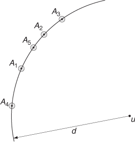
As explained above, path loss models have the purpose of estimating the intensity of the radio signal received at a certain distance from the transmitter when averaged overall a relatively small area. The geometric interpretation of path loss and shadowing is reported in Figure 2.1. Assume we have a wireless transmitter u, and let us focus our attention on what happens when the potential receiver is located at distance d from u, that is, somewhere on the large circle. Let us fix a certain position at distance d from u, say point A1. Experience teaches us that the intensity of the radio signal received at A1 might vary considerably if the position of A1 is slightly perturbed, due to so-called small-scale fading effects which we will describe shortly. To smooth such variations over a relatively small spatial scale, the intensity of the radio signal received at A1 is computed as the average of the intensity of the received signal when the position of the potential receiver is slightly changed around A1; say, in a disk of radius r, with r ![]() d, centered at A1 (shaded disk in Figure 2.1). Let
d, centered at A1 (shaded disk in Figure 2.1). Let ![]() denote this average value of the radio signal received at A1, and assume several such values
denote this average value of the radio signal received at A1, and assume several such values ![]() are sampled by randomly choosing positions on the circle of radius d centered at u. The log-distance path loss model with log-normal shadowing dictates that:
are sampled by randomly choosing positions on the circle of radius d centered at u. The log-distance path loss model with log-normal shadowing dictates that:
![]()
Figure 2.1 Geometrical interpretation of path loss and large-scale fading.
As commented above, experience has taught wireless communication engineers that the intensity of the radio signal often varies significantly even on a small spatial scale, for example, within the shadowed disk in Figure 2.1. This phenomenon, known as small-scale fading, is caused by the interference between two or more versions of the transmitted signal arriving at the receiver through different propagation paths, hence at slightly different times. Due to differences in amplitude and, most importantly, phase of the various versions of the signal received, the resulting combined radio signal in general displays considerable variations in both amplitude and phase depending on the distribution of the intensity and relative propagation time of the electromagnetic waves along the different paths. Thus, even slight changes in the propagation environment (e.g., because of movement of the receiver, or of an object in the environment) might cause very significant variations in the received radio signal power.
Small scale fading models have the goal of modeling the fluctuation of the received radio signal power around the mean value (as predicted by a path loss model) in either the (small scale) spatial or temporal domain. Well-known small scale fading models are the Ricean model, which models scenarios in which there is a dominant propagation path (LOS conditions), and the Rayleigh model, which is instead used when no dominant propagation path is present (no LOS conditions). The interested reader is referred to Molisch (2005) and Rappaport (n.d.) for descriptions of small scale fading models. In the remainder of this chapter, we will mostly ignore small scale fading effects, and restrict our attention to path loss models.
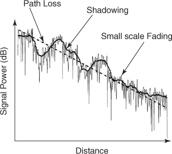
The compound effect of path loss, shadowing, and small-scale fading as the distance between transmitter and receiver increases is shown in Figure 2.2: path loss (dash–dotted plot) gives the decreasing trend of the signal intensity with distance; shadowing (bold curve) describes the variation of the actual received signal intensity around this trend, when averaged over short distances; finally, small-scale fading (light curve) gives the actual intensity of the received signal, considered as a variation over the superimposed effect of path loss and shadowing.
Figure 2.2 Compound effect of path loss, shadowing, and small-scale fading as a function of the separation distance between transmitter and receiver (courtesy of Konstantinos Mammasis).
2.2 The Communication Graph
The communication graph defines the topology of a wireless network, that is, the set of wireless links that nodes can use to communicate with each other. Given the discussion in the previous section, it is clear that the presence of a wireless link between a pair of units u and v depends on: (i) the location of u and v, and in particular their relative distance; (ii) the power used to transmit data; (iii) the data rate/coding scheme used to send data; (iv) the radio technology; and (v) the radio propagation environment.
To simplify the definition of the communication graph, in what follows we assume that the transmission power used to transmit data is fixed for each node u in the network. To further simplify presentation, and without loss of generality of the presented model, we further assume that the transmit power is the same for each node in the network, and we denote this transmit power value by Pt. Note that this is a simplification of reality, where network nodes can use transmit power control to dynamically change transmission power in order to adapt to actual radio channel conditions—transmit power control is a standard technique in cellular networks. Furthermore, in a network composed of heterogeneous devices it is very likely that the transmission power used by different devices, even if not dynamically changed, is set to different values. However, including transmit power control and heterogeneous transmission power values in the model of the communication graph introduced below is a straightforward exercise, which we leave to the interested reader—see also Chapter 2 of Santi (2005). In what follows we further assume that the data rate/coding scheme for each link is fixed and the same for all links; also, the features of the radio technology are incorporated in the thresholds (sensitivity and SNR threshold) used to determine existence/non-existence of a link. With all these simplifications, whether a link between units u and v exists becomes dependent only on (i) and (v) as described above.
Even if we consider a situation where only (i) and (v) play a role in determining the existence of a wireless link, the property defined as “a link between u and v exists” is time varying, that is, the link can exist at a certain time t, and it can no longer exist at a later time (t + 1). It is important to observe that, due to small-scale fading effects, the existence of a wireless link between u and v is a time-varying property even if the positions of u and v are fixed. However, small-scale fading effects are disregarded in the following to simplify the presentation. If such effects are disregarded, the existence of a wireless link becomes a time-varying property only in the presence of node mobility.
Concerning the propagation environment, we start by assuming deterministic path loss with a log-distance power model, for some value α > 1 of the distance–power gradient. In the last part of this section, we will generalize the model of the communication graph to random path loss models, bringing log-normal shadowing into the picture.
Let N be a set of wireless nodes, with |N| = n. Assume the nodes are located in a certain bounded region R, which for simplicity we assume is two dimensional (extension of the presented model to one- and three-dimensional domains is straightforward). Given any node u ∈ N, the location of u in R, denoted L(u), is the position of u in R, expressed in two-dimensional coordinates. Thus, we can define a function ![]() that maps a node u to its two-dimensional coordinates in R. In the case of mobile nodes—the scenario of interest in this book—the location function is redefined by adding a time parameter, that us, the location function becomes
that maps a node u to its two-dimensional coordinates in R. In the case of mobile nodes—the scenario of interest in this book—the location function is redefined by adding a time parameter, that us, the location function becomes ![]() . Summarizing, a mobile wireless network is represented by the pair M = (N, L), where N and L are defined as above.
. Summarizing, a mobile wireless network is represented by the pair M = (N, L), where N and L are defined as above.
Given a network M = (N, L), having fixed parameters of the radio link (data rate and coding scheme) and radio technology, disregarding small-scale effects, and given a value α > 1 for the distance–power gradient, the topology of the network at a certain time t is represented by the communication graph computed at time t, where the communication graph is defined as follows. The communication graph at time t is the undirected graph G(t) = (N, E(t)), where undirected edge (u, v) ∈ E(t) if and only if both conditions below are satisfied:
Note that, under our working assumption of homogeneous transmission power Pt, homogeneous radio technology, and same data rate/coding scheme on each link, the above conditions are satisfied for the wireless link between transmitter node u and receiver node v if and only if the same conditions are satisfied in the reverse link. In other works, the communication graph contains only symmetric (or bidirectional) wireless links.
Once specific values for α, β, and γ are set, conditions 1 and 2 above are equivalent to defining a transmission range r(α, β, γ)—the same for all the nodes– with the property that link (u, v) ∈ E(t) if and only if duv(t) ≤ r(α, β, γ), where duv(t) represents the distance between nodes u and v at time t. When the specific values of parameters α, β, and γ are not relevant, we will denote the transmission range simply by r. With all these simplifications, the communication graph as defined here becomes equivalent—once transmission range r is normalized to 1—to the notion of unit disk graph, which is well known in geometric graph theory (Clark et al. 1990). In a unit disk graph (UDG), a disk of unitary radius is centered at each node, and an edge between nodes u and v is added to the graph if and only if the disks centered at u and v intersect. An example of how the communication graph is computed given node positions and a transmission range r is shown in Figure 2.3.
Figure 2.3 A wireless network (top) and the corresponding communication graph (bottom). Transmission range of nodes is represented by a shaded disk.
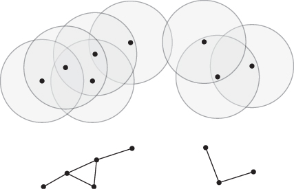
A communication graph is said to be connected at time t if and only if, for any two nodes u, v ∈ N, there exists a path in G(t) connecting u and v (and vice versa, given link symmetry). Note that the communication graph in Figure 2.3 is not connected, since nodes on the left hand side of the network cannot reach those on the right hand side.
The major shortcoming of the UDG model is the assumption of perfectly circular radio coverage. As discussed in the previous section, this assumption is hardly met in practice, especially in indoor and urban scenarios where shadowing and small-scale fading play a major role. While including accurate shadowing and small-scale fading models in the network model would make it extremely complex and dependent on scenario, generalizations of the UDG model aimed at accounting for irregular radio coverage areas have been recently proposed (Kuhn et al. 2008; Scheideler et al. 2008). In what follows we present the model introduced in Scheideler et al. (2008), which the authors prove to closely resemble log-normal shadowing.
The main idea of Scheideler et al. (2008) is to introduce a notion of cost related to an arbitrary node pair, and to introduce a link between two nodes if and only if the corresponding cost is below a certain threshold. More formally, consider any cost function ![]() with the property that there is a fixed constant θ ≥ 0 so that for all u, v ∈ N,
with the property that there is a fixed constant θ ≥ 0 so that for all u, v ∈ N,
The cost function c determines the transmission behavior of nodes, and parameter θ bounds the non-uniformity of the environment. In particular, a link between node u and v is considered to be present if and only if c(u, v) ≤ r, where r is a constant representing the transmission range. Notice that the model does not impose any other constraint on function c, such as being monotonic in the distance, to satisfy the triangle inequality, or symmetric.
In Scheideler et al. (2008), the authors show that, by suitably defining parameter eta, the cost function can be defined to closely resemble a specific propagation environment with log-normal shadowing. First, it should be noticed that, since the support of random variable LS = N(0, σ) modeling variation in path loss due to shadowing is infinite, the only way to make the cost model defined above resemble a log-normal shadowing environment is to let parameter θ grow to infinity, resulting in a model where nodes even arbitrarily close to each other might not be able to communicate, or where arbitrarily distant nodes might be able to communicate. In other words, the resulting model would correspond to a completely randomized propagation environment, which is not realistic as well. Thus, Scheideler et al. (2008) propose using a path loss model where the random variable modeling large-scale fading has bounded support. More specifically, it is assumed that large-scale fading is modeled by a random variable LS′ which takes values in [ − hσ, hσ] when expressed in dB, where h is a constant and σ is the standard deviation of LS = N(0, σ). The probability density function (pdf) of the newly defined random variable LS′ is obtained from the pdf LS by uniformly distributing the probability density of N(0, σ) falling outside [ − hσ, hσ] in the [ − hσ, hσ] interval. For instance, by setting h = 3 we get that only 0.0027 of the probability mass of variable LS = N(0, σ) falls outside the interval [ − 3σ, 3σ], and the pdf of LS′ is virtually indistinguishable from the pdf of LS.
The above-described bounded version of log-normal shadowing can be represented by setting parameter θ in Equation (2.3) equal to 10hσ/(10α) − 1, where σ and α are the parameters of the path loss model. For instance, by setting α = 3, σ = 6 dB, and h = 3, we obtain θ ≈ 1.5, implying that a transmission between nodes u and v is always successful when d(u, v) < 0.399r, and that a successful transmission can only occur at a distance less than or equal to 2.5r.
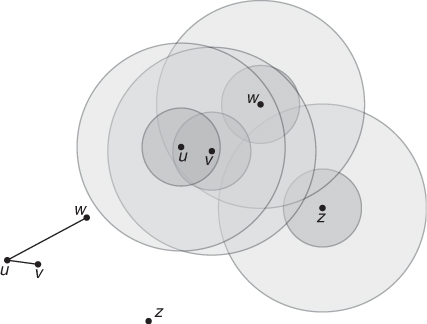
An example of a communication graph obtained with the cost model defined above is shown in Figure 2.4. Nodes within the dark shadowed disk centered at u (e.g., node v) always have a wireless link with u; nodes within the light shadowed annulus (e.g., node w) might have a link with u, as determined by the underlying bounded log-normal shadowing model; nodes outside the larger disk centered at u (e.g., node z) cannot have a link with u.
Figure 2.4 A wireless network (top) and the corresponding communication graph (bottom) obtained with a cost-based model.
In summary, the cost model proposed in Scheideler et al. (2008) can be used to model a bounded variant of the log-normal shadowing path loss model, under the assumption that the cost function c when defined for node pair (u, v) is defined as a random variable resulting from the product of a deterministic term equal to duv and a random term which has bounded log-normal distribution.
2.3 The Energy Model
One of the primary design concerns in a vast class of next generation wireless networks (e.g., wireless sensor and opportunistic networks) is the efficient use of energy. Thus, it is fundamental to model the node energy consumption accurately.
Depending on the scenario, next generation wireless networks can be composed of nodes of the most diverse type: laptops, cell phones, PDAs, smart appliances, tiny sensor nodes, and so on. Furthermore, for many application scenarios (e.g., opportunistic networks) the network can be composed of heterogeneous devices. Given this node diversity, a typical approach in the literature is to focus attention on the energy consumption of the wireless transceiver only.
Depending on the type of device, the amount of energy consumed by the transceiver varies from about 15% to about 35% of the total energy dissipated by the node. The former value refers to a laptop equipped with an IEEE 802.11 wireless card, while the latter is typical of a PDA device. An even higher portion of the total energy is consumed by the transceiver in a wireless sensor node.
Energy models for next generation wireless networks typically amount to estimating energy dissipation in the different operational modes of a wireless transceiver, which are:
Node energy consumption in the various operational modes is typically expressed using the sleep:idle:rx:tx power ratios, where the energy consumption in idle mode is conventionally assumed to be 1. Thus, an energy model is defined by assuming power x is consumed when the radio is receiving a message, power y is consumed when the radio is transmitting a message at full power Pt, and power z is consumed when the radio is in sleep mode (the actual values of x, y, and z depend on the specific wireless transceiver).
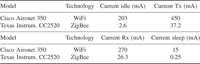
Typical values of current draw for different radio technologies are given in Table 2.2. Note that, if the wireless transceiver allows transmit power control, different transmit power modes (one for each specific value of the transmission power) might be defined, each resulting in a different power ratio.
Table 2.2 Current draw of typical WiFi and ZigBee products
Clark BN, Colbourn JC and Johnson DS 1990 Unit disk graphs. Discrete Mathematics 86, 165–177.
Kuhn F, Wattenhofer R and Zollinger A 2008 Ad hoc networks beyond unit disk graphs. Wireless Networks 14, 715–729.
Molisch A 2005 Wireless Communications. John Wiley & Sons, Ltd, and IEEE Press, Chichester.
Rappaport T n.d. Wireless Communications: Principles and Practice Second Edition. Prentice Hall, Upper Saddle River, NJ.
Santi P 2005 Topology Control in Wireless Ad Hoc and Sensor Networks. John Wiley & Sons, Ltd, Chichester.
Scheideler C, Richa A and Santi P 2008 An O(log n) dominating set protocol for wireless ad hoc networks under the physical interference model. Proceedings of ACM MobiHoc, pp. 91–100.