
Chapter 3
Mobility Models for Next Generation Wireless Networks
In the previous chapter, we motivated the importance of simulation in next generation wireless network analysis and introduced models for the radio channel, network topology, and energy consumption in a wireless node. In this chapter, we will focus on models of wireless node mobility, starting with motivating their importance within the network performance evaluation process. We will then extensively discuss the reasons why the existing know-how on mobility models for cellular networks cannot be applied (at least, directly) to model mobility in next generation wireless networks. Next, a taxonomy of existing mobility models for next generation wireless networks based on different criteria will be introduced. Finally, we will present the CRAWDAD web community resource for archiving mobility traces derived from real-world experiments and testbeds.
3.1 Motivation
We saw in the previous chapter that, given the difficulties related with realization, operation, and maintenance of testbeds, analysis and simulation play a fundamental role in next generation wireless network performance evaluation, especially when the network designer is interested in understanding network behavior when the number of nodes becomes large. Hence, suitable models must be developed to deal with the various aspects that might influence network performance; these models can then be combined and used to estimate expected network performance through either analysis or simulation.
Node mobility is a prominent feature of most of the next generation wireless network scenarios and applications briefly described in Chapter 1:
Summarizing, in the vast majority of next generation wireless network application scenarios, mobility not only is present, but plays a major role in governing network behavior and performance. This explains the extensive research efforts devoted to next generation wireless network mobility modeling in recent years, which is the focus of this book.
3.2 Cellular vs. Next Generation Wireless Network Mobility Models
Since node mobility is an important aspect also of more traditional types of wireless networks, such as cellular networks, the reader might be wondering why the extensive literature on cellular network mobility modeling cannot be applied—at least, directly—to next generation wireless networks. In this section, we will describe the main features of cellular network mobility models and explain why they are not suitable for modeling mobility in next generation wireless networks.
In a cellular network, space is divided into a well-organized cell structure, typically according to an hexagonal pattern as represented in Figure 3.1. A base station is located in each cell and is assumed to fully cover all nodes residing within its cell, that is, all nodes located in a cell can establish a direct wireless link with the corresponding base station.
Figure 3.1 A cellular network architecture.
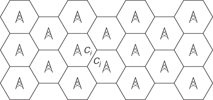
The performance of a cellular network, expressed for instance in terms of number of served clients and QoS parameters, depends greatly on the number of “active” nodes (i.e., customers making a call) residing in each cell, and how these numbers evolve over time. The number of active nodes in the various cells and their evolution over time depend on many factors, including node mobility. In particular, a call initiated in a certain cell Ci can be transferred to an adjacent cell Cj as the active node moves from Ci to Cj (see Figure 3.1). The process of transferring an active call between adjacent cells is called cell handoff, and it is a very critical operation in cellular networks, since handoff should be completed without interrupting the call and with minimal impact on QoS parameters. Another parameter influencing cellular network performance is the cell residence time, that is, the time that an active node is expected to spend in a certain cell, which is important for optimizing the allocation of radio resources in the cell. Cell handoff and residence time are not the only cellular network parameters influenced by node mobility, but they are sufficient to illustrate why cellular network mobility models cannot be directly used to analyze the performance of next generation wireless networks.
The effect of node mobility on cell residence time and handoff probability can be modeled and evaluated using a macro mobility model, operating at the spatial granularity of a network cell: what is relevant from the point of view of a network designer is not the actual trajectory that a specific active node follows, but the instants of time at which a node trajectory crosses the border of a cell. This is illustrated in Figure 3.2, which is adapted from Kim and Choi (2010): the trajectory of an active node is divided into a number of segments S1, …, Sk, corresponding to intervals of times in which the node resides in the same cell. The first segment is determined by the time interval elapsing between time t1 when the call is initiated and time t2 at which the node exits from the initial cell. Segments S2, …, Sk−1 are determined by cell crossing times t2, …, tk−1, while the last segment Sk is determined by the time interval elapsing between time tk−1 when the node enters the last cell and time tk when the node terminates the call.
Figure 3.2 Node mobility in a cellular network.
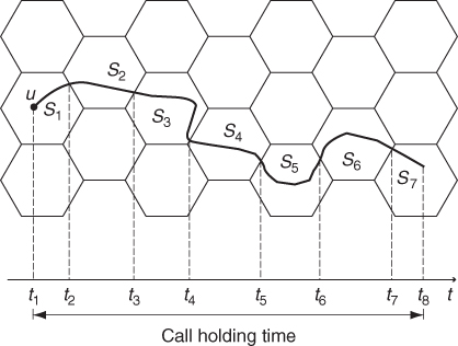
It is important to observe that, from the network designer's point of view, the relevant events related to a node mobility are the cell crossing times ti, as they determine cell residence time and handoff probability. On the other hand, the details of the trajectory that a node follows within a specific cell—that is, the position of node u within a time interval (t′, t′′), with ti < t′ < t′′ < ti+1 for some 1 ≤ i ≤ k − 1—has very little relevance from the network designer's point of view. In this case, the extreme case of a node moving within a single cell is seen as no mobility.
In the previous paragraph, we emphasized the word network when referring to a designer interested in characterizing macro-level node mobility, and stated that, from this designer's point of view, mobility of a node within a cell is not very relevant. Intra-cell mobility is instead of interest to the wireless communication engineer in the process of optimizing the quality of the radio transmission between the base station and the client node. However, as explained in Section 2.1, the effects of small-scale, intra-cell node mobility on link quality are typically considered in the definition of the radio channel model—more specifically in the definition of small-scale fading models.
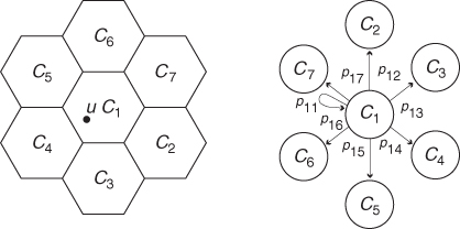
Macro-level node mobility in cellular networks is typically modeled using discrete-time Markov chains—see Appendix A.1 for a formal definition of Markov chains and their main properties—with states corresponding to cells, and transition probabilities corresponding to the probability of a node moving to another cell at the next time slot. In Figure 3.3, a portion of a cellular network is shown on the left hand side, with a node u located in cell C1 at time t. Under the quite common assumption that nodes can move only to adjacent cells, the right hand side of Figure 3.3 shows the portion of Markov chain representing possible transitions from state C1, and the respective probabilities. Thus, node u has probability p11 of remaining in cell C1 at time t + 1, and probability (1 − p11) of moving to another cell. In particular, node u moves to cell C2 with probability p12, to cell C3 with probability p13, and so on.
Figure 3.3 Portion of a cellular network (left) and portion of the corresponding Markov chain modeling node mobility between cells (right).
In the vast literature on cellular network mobility modeling, several Markov chain-based mobility models have been introduced, and their properties extensively studied. The interested reader is referred to Kim and Choi (2010) and references therein.
Cellular network mobility models as described above are not suitable for modeling mobility in next generation wireless networks for the following reasons:
3.3 A Taxonomy of Existing Mobility Models
In the previous section, we explained why cellular network mobility models cannot be directly applied to model mobility in next generation wireless networks. This fact, coupled with the paramount importance of mobility when studying next generation wireless network performance, explains the many efforts made in recent years by the research community to define and study suitable next generation wireless network mobility models. Surveys of this body of research work can be found in Bai and Helmy (2006), Camp et al. (2002), and Musolesi and Mascolo (2009). In this book, we will provide a more thorough and systematic treatment of this body of knowledge, which we will attempt to characterize and present as a scientific discipline rather than a collection of loosely related mobility models and results.
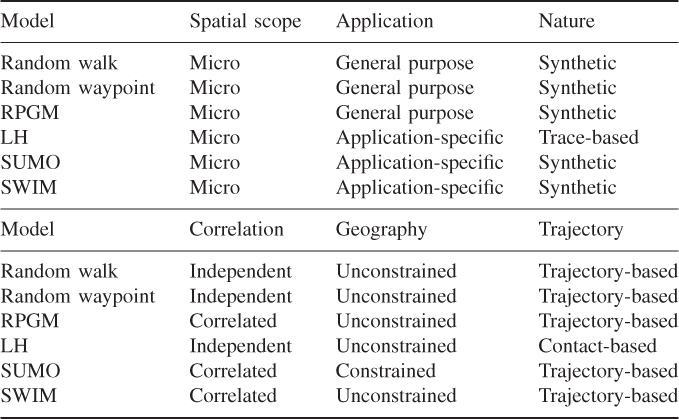
As a first effort in this direction, in this section we propose a taxonomy of existing mobility models—from now on, by the term “mobility model” we mean “mobility model for next generation wireless networks.” Instead of proposing a well-structured, hierarchical taxonomy with categories and subcategories, we present and describe extensively a set of independent criteria according to which mobility models can be classified. The criteria that will be used to classify existing mobility models are listed in Table 3.1, along with a classification of some of the mobility models which we will describe in this book according to these criteria.
Table 3.1 Classification of representative mobility models according to different criteria
3.3.1 Spatial Scope
The first criterion used to classify mobility models is spatial scope, as already described in the previous section. As commented above, given the relatively short transmission range typical of nodes in a next generation wireless network, all mobility models proposed in the literature aim at modeling mobility in a relatively small spatial scope, that is, with a spatial granularity in the order of a few tens of meters. Accordingly, mobility models for next generation wireless networks can be considered as members of the class of micro-mobility models (see Table 3.1).
3.3.2 Application Scenario
A second criterion useful for classifying mobility models is whether a model is tailored to a specific application scenario or not. In the former case, we use the term application-specific mobility model, while in the latter we use the term general-purpose mobility model.
General-purpose mobility models are typically synthetic (for a definition of synthetic mobility model see Section 3.3.3) models defined through simple mathematical rules. Simplicity is the primary reason why general-purpose mobility models have been used so extensively in the next generation wireless networking literature. In fact, the simple mathematical rules used to define node mobility can be easily embedded into a wireless network simulator, thus significantly easing the complex task of simulating wireless network behavior. A further boost to usage of general-purpose mobility models is that an implementation of the most representative models in this class is included in recent releases of widespread wireless network simulators, such as Ns2 (Team 2011d), GloMoSim (Team 2011b), and GTNetS (Team 2011c). Another factor contributing to the success of general-purpose mobility models is that they are among the few mobility models that, due to their simplicity, allow derivation of theoretical, foundational results about mobile networks.
Representative examples of the class of general-purpose mobility models are the family of random walk models, which will be described in Chapter 4, and the random waypoint mobility model (Johnson and Maltz 1996), which is by far the most commonly used mobility model in ad hoc network simulation.
The major shortcoming of general-purpose mobility models comes from the primary reason for their widespread use, namely, their simplicity. Since these models are defined through simple mathematical rules, it is very difficult to account for the many factors influencing mobility in a real-world application scenario. For instance, general-purpose mobility models typically assume that nodes move in a spatial domain without any constraint regarding the trajectories they can follow—that is, they are unconstrained mobility models, see Section 3.3.5. Except for a few situations (e.g., people or animals moving in a vast, unobstructed space), movement is instead highly constrained in the real world: individuals move along sidewalks and pathways, cars move along roads, etc.
Given these shortcoming, several mobility models have been proposed with the explicit purpose of modeling a specific application scenario with a related network architecture. Mobility models specifically designed for WLAN environments, vehicular networks, and so on, have been introduced in the literature in recent years. Unfortunately, tailoring a mobility model to a specific application scenario often comes at the expense of significantly complicating the definition of the model, making the simulation and (even more) the analysis task much more challenging than in the case of general-purpose mobility models.
3.3.3 Nature
Mobility models can be classified also according to whether they are synthetically defined through simple mathematical rules, or rather they are stochastically defined to resemble mobility patterns observed in real-world data traces. In the former case, we use the term synthetic mobility model, while in the latter case we use the term trace-based mobility model.
In a synthetic mobility model, rules are defined to determine the initial position of a node, as well as its trips, where a trip is typically characterized by a starting point, an endpoint, a trajectory connecting the starting and endpoints, and a velocity. On the other hand, in trace-based mobility models, what is relevant are not the actual trajectories followed by the nodes, but rather their contact patterns, which should resemble as closely as possible those observed in representative traces collected in real-world experiments. In this respect, trace-based mobility models display some resemblance to cellular network mobility models, since in these models also the specific trajectory followed by a node is not of interest to the network designer. However, the spatial scope of trace-based mobility models is typically small, so differently from cellular network mobility models they belong to the class of micro-level mobility models.
3.3.4 Correlation
Another criterion according to which mobility models can be classified is whether the movement of a node is independent of or correlated with the movement of other nodes. In the former case, we use the term independent mobility model, while in the latter case we use the term correlated mobility model.
In an independent mobility model, the movement of a node is stochastically independent of the movement of any other node in the network. Typically, movement patterns of different nodes are not only independent, but also stochastically equivalent. In other words, the probabilistic rules governing node mobility are the same for all the nodes, resulting in the same stochastic behavior of all network nodes.
Anyone who has some experience in the simulation and analysis of relatively complex systems will understand the importance of the independence assumption when simulating or analyzing the performance of a wireless network: both simulation and analysis are significantly simplified if nodes move in a stochastically independent fashion. Unfortunately, the mobility of nodes is indeed highly correlated in my real-world situations. Think for instance of a typical vehicular network scenario: well-defined traffic rules strongly correlate the movement of a vehicle with those of surrounding vehicles. Another example is instances of group mobility, such as a scenario where a group of tourists follows a tourist guide. Correlated mobility models have been introduced to model situations in which the movement of a node is highly correlated with, if not completely dependent on, the movement of other nodes in the network.
3.3.5 Geography
A further criterion distinguishing mobility models is whether node mobility is geographically constrained or not. In the former case, we use the term geographically constrained mobility model, while in the latter case we use the term unconstrained mobility model.
In unconstrained mobility models, nodes are free to move everywhere within a predefined geographical domain representing the range of possible node movements. Typical representatives of the class of unconstrained mobility models are general-purpose, synthetic—hence, simple—mobility models. While simplicity is definitely a positive feature of a mobility model, unconstrained mobility models typically share with general-purpose, synthetic models also the major shortcoming of being scarcely representative of many real-world scenarios, in which node mobility is indeed highly geographically constrained. Examples of geographically constrained mobility abound: vehicles moving along roads, individuals moving along sidewalks and pathways, etc.
It is interesting to observe the relation between geographical constraints and correlation of node movements: while correlation of node movements might indeed be imposed by geographical constraints, a geographically constrained mobility model is not necessarily correlated. For instance, when considering mobility models for vehicular networks, vehicles can be constrained to move along roads, but traffic rules can be ignored—like considering vehicles as “transparent” entities to avoid accidents.
3.3.6 Trajectory
Finally, another criterion that can be used to classify mobility models is whether they generate explicit trajectories for each node, or rather generate traces of mutual contacts between nodes. In the former case, we use the term trajectory-based mobility model, while in the latter we use the term contact-based mobility model.
While node trajectories, coupled with a notion of transmission range, can be used to generate node contact patterns if needed, the main difference between the two classes of models is that trajectory-based mobility models explicitly model and give access to a notion of node trajectory, while in contact-based mobility models no notion of node trajectory is explicitly or implicitly used to generate the contact traces which are returned as an output of the model. Contact traces are typically obtained through stochastically modeling the occurrence/disappearance of links between pairs of nodes, using Markov chain-based models.
As the reader might have guessed, trace-based mobility models typically do not explicitly represent node trajectories, but rather their contact patterns; that is, they typically belong to the class of contact-based mobility models.
3.4 Mobility Models and Real-World Traces: The CRAWDAD Resource
Mobility models have the main goal of mimicking certain types of mobility (human, vehicular, animal, etc.), or at least of resembling their most distinguishing features. Thus, the ultimate way of assessing the “performance” of a mobility model is to compare the mobility traces it generates with those collected in real-world mobility experiments for the relevant mobility scenarios.
Mobility traces collected in such experiments are a fundamental resource for next generation wireless network designers. On the one hand, they can be used to validate and/or fine-tune artificial mobility models as described above. On the other hand, they can also be directly used in the network performance evaluation process, for example, by feeding wireless network simulators with the collected mobility traces. However, real-world mobility traces should be seen as complementing, not replacing, the role of artificial mobility models in the network performance evaluation process, for the following reasons:
While many of the issues listed above are in a sense intrinsic to the mobility data collection task, significant efforts have been recently undertaken in the research community to make a large number of mobility traces publicly available. The most important initiative in this direction is the Community Resource for Archiving Data At Dartmouth (CRAWDAD) (Team 2011a), a project led by David Kotz of Dartmouth College, USA. The project started in 2004 with a data collection campaign of syslog, SNMP, and tcpdump data from the WLAN installed at Dartmouth College. Since then, the project has evolved to become a community resource for archiving mobility traces related to wireless networks.
The homepage of the CRAWDAD website is displayed in Figure 3.4. CRAWDAD resources amount not only to a large set of publicly available mobility traces—as of the beginning of 2012, 78 traces are available—but also to a set of tools for visualizing and processing these traces—23 tools are available—and to browsing tools allowing navigation of the traces by keywords, etc.
Figure 3.4 The CRAWDAD website.
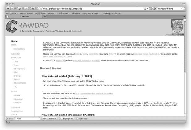
In recent years, CRAWDAD has become a very valuable resource for next generation wireless network designers, as witnessed by the fact that—as of the beginning of 2011—more than 500 scientific papers using CRAWDAD mobility traces have been published.
3.5 Basic Definitions
In this section, we provide the basic definitions and terminology that will be used to describe the various mobility models presented in this book. Most of these definitions apply to the class of synthetic mobility models which, as can be seen from Table 3.1, covers the vast majority of mobility models commonly used in the literature.
A synthetic mobility model can be formally defined through a set of rules specifying the following:
A very important notion in mobility modeling is that of stationary node spatial distribution. Consider a certain synthetic mobility model ![]() , and let X0 be a variable denoting the position of a node u at time 0. Note that X0 is determined according to the rules for initial node positioning as defined in
, and let X0 be a variable denoting the position of a node u at time 0. Note that X0 is determined according to the rules for initial node positioning as defined in ![]() . In particular, if X0 is randomly selected, X0 is a random variable with values in R, with f0 being the corresponding pdf. As node u starts moving, its position varies within R. Let X(t) denote the position of u at time t > 0. If trips are randomly selected, X(t) also can be considered as a random variable defined within the spatial domain R. Let ft denote the pdf of random variable X(t). Assuming for simplicity that R is a two-dimensional domain, function ft(x, y) corresponds to the probability density of finding node u exactly at position (x, y) at time t. Note that, given the definition of mobility model
. In particular, if X0 is randomly selected, X0 is a random variable with values in R, with f0 being the corresponding pdf. As node u starts moving, its position varies within R. Let X(t) denote the position of u at time t > 0. If trips are randomly selected, X(t) also can be considered as a random variable defined within the spatial domain R. Let ft denote the pdf of random variable X(t). Assuming for simplicity that R is a two-dimensional domain, function ft(x, y) corresponds to the probability density of finding node u exactly at position (x, y) at time t. Note that, given the definition of mobility model ![]() , the support of both f0(x, y) and ft(x, y) is contained in R.
, the support of both f0(x, y) and ft(x, y) is contained in R.
![]()
that is, if, ![]() . In such a case, function
. In such a case, function ![]() is said to be the stationary node spatial distribution of
is said to be the stationary node spatial distribution of ![]() .
.
It is important to observe that the stationary node spatial distribution of a mobility model might be different from the initial node spatial distribution, that is, ![]() in general.
in general.
Bai F and Helmy A 2006 A survey of mobility modeling and analysis in wireless ad hoc networks. Wireless Ad Hoc and Sensor Networks. Springer, Berlin.
Camp T, Boleng J and Davies V 2002 A survey of mobility models for ad hoc network research. Wireless Communications and Mobile Computing 2, 483–502.
Johnson D and Maltz D 1996 Dynamic source routing in ad hoc wireless networks. Mobile Computing, pp. 153–181. Kluwer Academic, Dordrecht.
Kim K and Choi H 2010 A mobility model and performance analysis in wireless cellular network with general distribution and multi-cell model. Wireless Personal Communications 53, 179–198.
Musolesi M and Mascolo C 2009 Mobility models for system evaluation. State of the Art on Middleware for Network Eccentric and Mobile Applications. Springer, Berlin.
Team C 2011a http://crawdad.cs.dartmouth.edu/index.php.
Team G 2011b http://pcl.cs.ucla.edu/projects/glomosim/.
Team G 2011c http://www.ece.gatech.edu/research/labs/MANIACS/GTNetS/.
Team N 2011d http://www.isi.edu/nsnam/ns/.
Team R 2006 http://reality.media.mit.edu/.