Chapter 12

Vehicular Networks: Macroscopic and Microscopic Mobility Models

Modeling mobility in a vehicular network is a very challenging task. In fact, vehicular mobility displays several features that, on the one hand, can be difficult to model and, on the other hand, have a deep impact on a vehicle's mobility behavior. Examples of distinguishing features of vehicular mobility are:

1. Geographically constrained movements: vehicles are (luckily!) not allowed to move arbitrarily in the space, but are forced to move along pre-existing paths—the roads. Hence, geographically constrained movement is a very important feature of vehicular mobility, which cannot be overlooked in the definition of the mobility model if an acceptable level of realism is sought.
2. Obedience to traffic rules: very strict rules govern movement of vehicles along roads, such as speed limits, traffic junction rules, lane changing rules, etc. Thus, at least the most representative such rules should be incorporated into the mobility model in order to improve accuracy.
3. Driver behavior: different drivers might display very different driving styles concerning, for example, willingness to respect traffic rules, aggressive/non-aggressive driving behavior, etc. Including driver behavior in the mobility model is perhaps the most difficult task in vehicular mobility modeling, which explains why a driver behavioral model is often not included in the vehicular model definition. However, at least for certain applications (e.g., when the mobility model is used to assess the effectiveness of active safety applications in reducing the number of road accidents), driver behavior should not be disregarded in the definition of the model.

Given these features, it is evident why the “model accuracy” vs. “simulation running time” tradeoff, which is present in next generation wireless network mobility modeling in general, becomes especially critical in vehicular network models. On the one hand, using simplistic (but fast!) mobility models typically generates highly inaccurate simulation results, due to the fact that some of features 1, 2, or 3 above are not included in the model. On the other hand, a full-fledged vehicular mobility model including accurate road maps, traffic rules, and driver behavior models is typically cumbersome and computationally intensive, and difficult to use in vehicular network simulation. Thus, an adequate tradeoff between model accuracy and simulation running time should be carefully evaluated, depending on the network designer's needs.

One possible way of addressing this tradeoff is to take into consideration the geographical scope of interest. According to geographical scope, vehicular mobility models can be classified as macro- or micro-models. In this chapter, we will briefly describe the main features of models in each of these classes.

12.1 Vehicular Mobility Models: The Macroscopic View

Macroscopic vehicular mobility models are used to model traffic flow in relatively large geographical regions—in the order of hundreds or even thousands of square kilometers. Macroscopic mobility models are mostly used by transportation engineers to estimate the amount of traffic flowing along the main roads in a region of interest. In turn, accurate traffic flow estimates can be used, for example, to optimize road traffic management, to study the effects of introducing new arterial roads, etc.

Given the relatively large geographical scope of interest, vehicular mobility is modeled at a coarse granularity. In particular, individual vehicles are not modeled; instead, relationships between traffic flow characteristics of interest in the road network. such as vehicle density, mean speed, etc., are modeled through a suitably defined system of partial differential equations. While driver behavior is typically not modeled in macroscopic mobility models, some traffic rules such as speed limits can be used as constraints on the system of equations modeling traffic flow in the road network.

The process of simulating vehicular mobility using a macroscopic mobility model is typically composed of four steps, as depicted in Figure 12.1:

1. Map creation: in this step, the region of interest is subdivided into a number of subregions, corresponding, say, to neighborhoods of a city, suburbs, villages, etc.; typically, a center of gravity is defined for each subregion, called the point of interest in the following. Also in this step, a map of the main roads connecting the various points of interest is created. An example of a macroscopic mobility map is shown in Figure 12.2.
2. Definition of the traffic demand matrix: in this step, a traffic demand matrix, T, is defined. T is an m × m matrix, where m is the number of points of interest in the region, and element (tij) represents the amount of traffic originating at the ith point of interest which is destined for the jth point of interest. Typically, the traffic demand matrix is enriched with temporal information, that is, the amount of traffic generated at a certain point i and destined for point j at different times of the day is defined. Since the traffic demand matrix constitutes the input to the macroscopic vehicular traffic model, it is important that the matrix is generated in an accurate way. This is typically done by combining usage of statistical data such as density of population, density of workplaces, etc., with samples of traffic measurements.
3. Route assignment: after the traffic demand matrix is defined and traffic demands at the various points of interest are generated, a routing algorithm must be defined to route traffic from origin to destination. This is typically done using the well-known Dijkstra shortest path algorithm.
4. Trip phase: when the three steps above have been performed, the actual simulation of traffic flow can start, and statistics of interests to the designer (e.g., average trip time, average and maximum flow on the roads, average travel speed, etc.) can be computed.

Figure 12.1 The four steps in macroscopic vehicular mobility simulation.

12.1

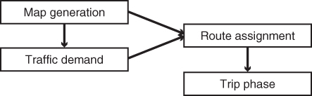
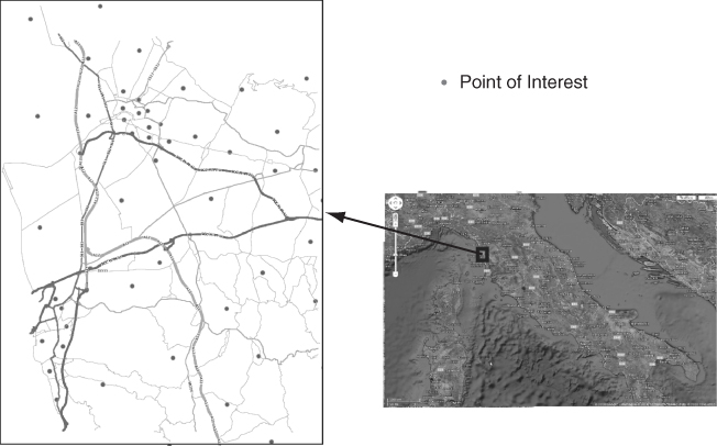
Figure 12.2 Example of a macroscopic mobility map of a region surrounding the city of Pisa, Italy (courtesy of Aleph SrL).

12.2

If the goal is, for instance, to estimate the impact on traffic of introducing a new road in the road system, the four-step process above can be repeated several times using different maps, until the “optimal” location of the new road is identified.

Given the relatively large geographical scope and lack of modeling individual vehicles, macroscopic mobility models are not very useful in vehicular network simulation, other than generating realistic traffic input values for microscopic mobility models (see next section). For this reason, in the following we will restrict our attention to the class of microscopic mobility models, which are briefly introduced in the next section and treated in detail in the next chapter.

12.2 Vehicular Mobility Models: The Microscopic View

Unlike macroscopic models, microscopic mobility models aim to give a detailed view of vehicular mobility, where the behavior of a single vehicle is modeled. Clearly, given that each vehicle traveling on the road is modeled, with current computational capabilities the simulation of a moderate number of vehicles (in the order of several thousand at most) can be undertaken. So, unless a scenario with very low vehicle density is modeled, this upper bound on the number of modeled vehicles imposes an upper bound on the size of the geographical region of interest. With current technology, microscopic mobility models can be used to simulate regions of the size of a large metropolitan area (tens of square kilometers).

The necessary steps for simulating vehicular mobility with a microscopic mobility model are similar to those for macroscopic simulation:

1. Map generation: the first step consists of acquiring or generating a digitized road map of the region of interest. In contrast to macroscopic models, the digital map is typically quite accurate, including not only main roads but also secondary ones. The level of detail of a digital map used in microscopic vehicular mobility models is similar to the one provided by Web-based tools such as Google Maps (Google 2011) or MapQuest (MapQuest 2011) at a level close to the maximum level of detail—see Figure 12.3 for an example.
2. Definition of the traffic demand: similar to the macroscopic case, traffic demands should be defined. However, the relatively small geographical scope of interest dictates some changes on how traffic demand values are generated. First, a typical assumption in microscopic modeling is that traffic can originate and be destined for outside the simulated region. In the usual approach, ingress/egress points at the borders of the region of interest are defined. Then, traffic demands are generated at ingress points and/or points of interest within the region, with destinations defined to be either egress points or another point of interest within the map. In order to generate realistic estimates of traffic originating and destined for outside the simulated region, the output of the macroscopic mobility model can be used to integrate the relatively small road system of interest with regional-scale traffic.
3. Route assignment: this step is also similar to the corresponding step in macroscopic models, the only relevant difference being that now routes are defined at the granularity of a single vehicle. That is, for each vehicle, given the trip origin, destination, and starting time as defined in the traffic demand matrix, a best route to a destination is computed using a Dijkstra-like shortest (or fastest) path algorithm.
4. Trip phase: when the map has been generated, the traffic demand defined, and the routes computed, the actual simulation of vehicular mobility can start, with relevant statistics such as average travel time (at single-vehicle granularity), average travel speed, and so on. It is important to observe that, different from macroscopic models, in microscopic mobility models traffic rules (lane changing, intersection rules, overtaking, etc.), and sometimes even driver behavior models, are included in the model definition. This implies that the movement of a vehicle is directly influenced by the movement of other vehicles. Hence, a supposedly best route as computed by the routing algorithm in the third step might turn out to be sub-optimal once the trip takes place due to interactions with other vehicles.

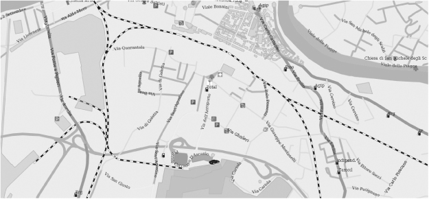
Figure 12.3 Example of a microscopic mobility map, reporting a portion of the city of Pisa, Italy (courtesy of Francesca Martelli).

12.3

12.3 Further Reading

As mentioned at the end of Section 12.1, in the next chapter we will describe in detail some representative microscopic mobility models. The reader interested in gaining a better understanding of macroscopic vehicular mobility models (also called traffic flow models) is referred to the several surveys (Bellomo et al. 2002; Coscia et al. 2007) and books (Kerner 2009) on the topic.

References

Bellomo N, Delitala M and Coscia V 2002 On the mathematical theory of vehicular traffic flow I: Fluid dynamic and kinetic modeling. Mathematical Models and Methods in Applied Sciences 12, 1801–1843.

Coscia V, Delitala M and Frasca P 2007 On the mathematical theory of vehicular traffic flow II: Discrete velocity kinetic models. International Journal of Non-Linear Mechanics 42, 411–421.

Google 2011 http://maps.google.com.

Kerner B 2009 Introduction to Modern Traffic Flow Theory and Control. Springer, Berlin.

MapQuest 2011 http://www.mapquest.com.

..................Content has been hidden....................

You can't read the all page of ebook, please click here login for view all page.
Reset
3.145.35.194