Appendix A
Elements of Probability Theory
In this appendix, we report basic notions of probability theory and stochastic process theory. The material of this appendix is based on Feller (1957), on Appendix B.1 of Santi (2005), and on online resources such as Wikipedia and Wolfram MathWorld.
A.1 Basic Notions of Probability Theory
Definition A.1 (Sample space)
A sample space Ω is a set representing all possible outcomes of a certain random experiment. A sample space is discrete if it is composed of a finite number of elements (e.g., outcomes of a coin toss experiment), or of infinitely many elements that can be arranged into a simple sequence e1, e2, ….
Definition A.2 (Random variable
A random variable X is a function defined on a sample space. If the sample space on which X is defined is discrete, X is said to be a discrete random variable.
Examples of random variables are the number of heads in a sequence of k coin tosses (discrete random variable), the position of a certain particle in a physical system, the position of a node moving according to a certain mobility model at a certain instant of time, and so on.
Definition A.3 (Probability distribution)
Let X be a discrete random variable, and let Ω = {x1, x2, …, xj, …} be the set of possible values of X. The function

is called the probability distribution (also called probability mass function) of the random variable X, where, for all i, f(xi) ≥ 0 and ∑if(xi) = 1.
Definition A.4 (Event and probability)
Let Ω = {x1, x2, …, xj, …} be a discrete sample space, and let f() be a probability distribution on Ω. An event is defined as any subset E of the sample space Ω. The probability of event E is defined as
Definition A.5 (Probability density function)
A probability density function (pdf) on

is a function such that
Similarly, with a fixed integer
d > 1, a pdf on

is a function such that
Definition A.6 (Continuous random variable
A random variable
X taking values in

is
continuous if and only if there exists a pdf
f on

such that
for any
a <
b. Function
f is called the
density of the random variable
X. A similar definition applies to random variables taking values in

, for some integer
d > 1.
Definition A.7 (Distribution function)
Let
X = (
X1, …,
Xd) be a continuous random variable taking values in

, for some integer
d ≥ 1. The function
where f(y1, …, yd) is the density of X, is called the (cumulative) distribution function of the random variable X. Function f is called the density of the random variable X.
Definition A.8 (Complementary cumulative distribution function)
Let
X = (
X1, …,
Xd) be a continuous random variable taking values in

, for some integer
d ≥ 1. The function
where f(y1, …, yd) is the density of X, is called the complementary cumulative distribution function of the random variable X.
Definition A.9 (Support of a pdf)
The support of a pdf
f on

, for some integer
d ≥ 1, is the set of points in

on which
f has positive value. Formally,

Clearly,
Definition A.10 (Asymptotic distribution)
A sequence X1, X2, …, Xn, … of continuous random variables, with distribution functions F1, F2, …, Fn, …, is said to converge in distribution to a certain random variable X with distribution F if and only if
at every continuity point x of F(x). If sequence {Xn} converges in distribution to a certain random variable X with distribution F, we say that F is the asymptotic distribution of {Xn}.
Definition A.11 (The a.a.s. and w.h.p. event)
Let En be a random variable representing a random event which depends on a certain parameter n. We say that the event represented by En holds asymptotically almost surely (a.a.s.) if
We say that the event holds with high probability (w.h.p.) if
Note that the fact that an event holds w.h.p. implies that the same event holds a.a.s.
Definition A.12 (Stochastic process)
Given a sample space Ω, a stochastic process is a collection of random variables taking value in Ω indexed by a set T of time instants. Formally, a stochastic process S is a collection {St:t ∈ T} where random variables St take values in Ω.
Examples of stochastic processes are the sequence of trip lengths of a mobile node, the sequence of statuses of a communication link (active or inactive) between two nodes in a network, and so on. A special class of stochastic processes are Markov chains, which will be formally defined in Section A.3.
Definition A.13 (Stationary process)
Let
S = {
St:
t ∈
T} be a stochastic process, and let
be the cumulative distribution function of the joint distribution of variables {
St} at time
t1 + τ, …,
tk + τ. Process
S is said to be
stationary if and only if, for all
k ≥ 1, for all τ > 0, and for all
t1, …,
tk,

Intuitively speaking, a stochastic process is stationary if the joint probability distribution of the observed random variables, and hence statistical properties such as mean and variance, do not change with time. A related notion for stochastic processes is that of ergodicity, which refers to the fact that the statistical properties of a (stationary) stochastic process can be deduced from sampling a large group of identical, independent instances of the observed process at a single time instant. Below we present the formal definition of mean ergodicity, a property used, for example, in the characterization of the node spatial distribution of mobility models. The more general notion of ergodicity is cumbersome to define, and it is therefore not reported here.
Definition A.14 (Mean ergodic process)
Let S = {St:t ∈ T} be a stochastic process, and let E[St] denote the expected value of St computed in two possible ways:
and
where, for any
fixed value of
t,

denotes the
ith independent instant of process
S at time
t. If process
S satisfies the
mean ergodic property, then
E[
St] =
Ee[
St].
A.2 Probability Distributions
Definition A.15 (Discrete uniform distribution)
Let X be a random variable taking values in Ω = {x1, …, xk}, for some integer k > 0. Random variable X is said to have uniform distribution if and only if its probability mass function satisfies P(X = xi) = 1/k, for each i = 1, …, k. A discrete random variable with uniform distribution is called a (discrete) uniform random variable.
Definition A.16 (Continuous uniform distribution)
Given an interval [
a,
b] on

, with
a <
b, the
uniform distribution on [
a,
b] is defined by the following probability density function:
The uniform distribution on arbitrary d-dimensional rectangles is defined similarly. A continuous random variable with uniform distribution on a certain (d-dimensional) interval is called a (continuous) uniform random variable.
Definition A.17 (Poisson process and distribution)
Let us consider a discrete random variable X(t), counting the number of events (e.g., arrival of telephone calls) occurring in the time interval [0, t]. If the following properties hold:
(a) the probability of occurrence of the observed events does not change with time, and
(b) the probability of occurrence of the observed events does not depend on the number of events occurred so far,
then the corresponding random process is called a Poisson process. In a Poisson process, the number of events counted after time t follows the probability function
for some constant λ > 0. Parameter λ is called the intensity of the Poisson process. The above probability function is called a Poisson distribution of parameter λ. A random variable with a Poisson distribution is called a Poisson random variable.
Definition A.18 (Normal distribution)
The
normal (or Gaussian) distribution on

of parameters μ (mean) and σ (standard deviation) is defined by the following probability density function

:
The normal distribution on

, for some integer
d > 1, is defined similarly. A random variable with a normal distribution is called a
normal random variable.
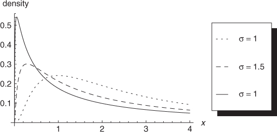
Definition A.19 (Log-normal distribution)
The
log-normal distribution on

of parameters μ (mean) and σ (standard deviation) is defined by the following probability density function:
The log-normal distribution on

, for some integer
d > 1, is defined similarly. A random variable with a log-normal distribution is called a
log-normal random variable.
The shape of the log-normal distribution with μ = 1 and different values of the standard deviation σ is shown in Figure A.1.
Definition A.20 (Exponential distribution)
The
exponential distribution on

of parameter λ (called
rate parameter) is defined by the following probability density function:
A random variable with an exponential distribution is called an exponential random variable.
The exponential distribution and Poisson process are related as follows: the time between two consecutive events in a Poisson process of intensity λ is an exponentially distributed random variable of rate λ.
Definition A.21 (Power-law distribution)
In the most general sense, a
power-law distribution on

is characterized by a probability density function (or probability mass function in the discrete case) of the following form:
where α > 1 is the slope parameter and L(x) is a slowly varying function, that is, a function such that limx→∞L(tx)/L(x) = 1, for any constant t.
The most interesting property of a power-law distribution is scale invariance, which states that scaling the argument of the function results in a proportional scaling of the density function itself. In formulas, if f is a power law of slope parameter α, then
Examples of probability distributions belonging to the class of power laws are presented in the following.
Definition A.22 (Power-law distribution with exponential cutoff)
A
power-law distribution with exponential cutoff on

is characterized by a probability density function (or probability mass function in the discrete case) of the following form:
where α > 1 is the slope parameter, L(x) is as defined above, and λ > 0 is the decay parameter of the exponential cutoff.
Note that in the power-law distribution with exponential cutoff the exponential decay term e−λx overwhelms the power-law behavior for large values of x, implying that the scale invariance property no longer holds.
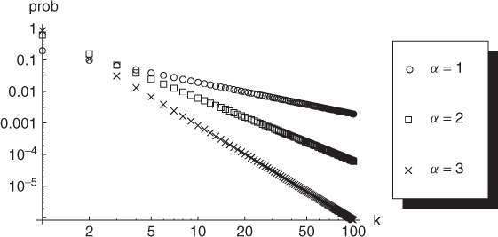
Definition A.23 (Zipf's law)
Let X be a discrete random variable defined on sample space Ω = {1, …, N}, and assume without loss of generality that elements in Ω are ordered from the most probable to the less probable outcomes of X; that is, Prob(X = 1) ≥ Prob(X = 2) ≥ …. We say that variable X obeys Zipf's law of slope parameter α if and only if
where
is the
Nth generalized harmonic number.
Zipf's law is typically used to model the uneven popularity of interests in a population, such as the popularity of multimedia files in a peer-to-peer file sharing application. Examples of Zipf's law with different slope parameters are given in Figure A.2. Notice that both axes are in logarithmic scale. In fact, log–log plots are commonly used to display power laws, since a power-law function corresponds to a linear function in log–log scale.
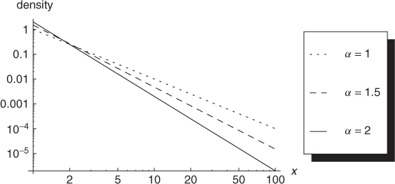
Definition A.24 (Pareto distribution)
Let X be a random variable taking values in [xm, + ∞), for some xm > 0. The random variable X is said to obey a Pareto distribution if and only if its probability density function is defined as follows:
where α > 0 is the slope parameter. A random variable with a Pareto distribution is called a Pareto random variable.
The Pareto distribution can be considered as the continuous counterpart of the Zipf's law distribution. Examples of a Pareto distribution with xm = 1 and different slope parameters are given in Figure A.3.
Definition A.25 (Truncated Pareto distribution)
Let X be a random variable taking values in [xm, xM], for some 0 < xm < xM. The random variable X is said to obey a truncated Pareto distribution if and only if its probability density function is defined as follows:
where α > 0 is the slope parameter.
A.3 Markov Chains
Definition A.26 (Markov chain)
A
Markov chain is a stochastic process where the random variables
X1,
X2, … in the sequence represent a discrete set
of possible
statuses, and where the probabilities governing transitions between states satisfy the
Markov property (also known as
memoryless property). The set

of possible states is called the
state space, and it is the sample space for each of the
Xi. The Markov property states that the probability of making a transition into any state
Si in the state space at time
t depends only on the status of the chain at time (
t − 1). Formally,

for any time
t > 0, where

.
Note that the state space in the Markov chain can be formed by a finite number or an infinite but countable number of elements.
Definition A.27 (Time-homogeneous Markov chain)
A time-homogeneous Markov chain is a Markov chain where transition probabilities do not change with time. Formally,

for any time
t > 0, where

.
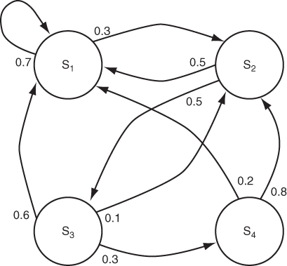
Time-homogeneous Markov chains with finite state spaces can be pictorially described by a directed graph  , where directed edge (xi, xj) ∈ E is labeled with transition probability pij = P(X1 = xj|X0 = xi) > 0 (edges are omitted for transitions occurring with zero probability). The pictorial representation of a four-state Markov chain is shown in Figure A.4. Note that the sum of the weights on the outgoing edges of each node is 1. In formulas,

for any

. The transition probabilities can be summarized in the
transition matrix Π = (
pij). Since the transition probabilities are time-invariant, the
k-step transition probabilities can be computed as Π
k, that is, the
kth power of the transition matrix Π.
Definition A.28 (Accessible state and communicating class)
A state

is said to be
accessible from state

if a chain started in state
Sj has non-zero probability of making a transition into state
Si at some point in time. Formally, a state
Si is accessible from
Sj if and only if
for some
t > 0. A state
Si is said to
communicate with state
Sj if and only if
Si is accessible from
Sj and vice versa. A set of states

is a
communicating class if, for every

,
Si and
Sj communicate, and no state in

communicates with any state in

.
Definition A.29 (Irreducible Markov chain)
A Markov chain is irreducible if its state space is a single communicating class.
Informally speaking, a Markov chain is irreducible if it is possible to make a transition into any state, starting from any state. The Markov chain represented in Figure A.4 is irreducible. In fact, starting from S1 it is possible to make a transition into S1 (in one step), into S2 (in one step), into S3 (in two steps, through state S2), and into S4 (in three steps, through states S2 and S3). The same transition applies starting from any other state.
Definition A.30 (Periodicity)
A state

has period
k if, starting from
Si, any return to state
Si must occur in multiples of
k time steps. If
k = 1, the state is said to be
aperiodic. Otherwise, it is said to be
periodic of period k. A Markov chain is said to be
aperiodic if all its states are aperiodic.
For instance, state S1 in the Markov chain of Figure A.4 is aperiodic, since there is a non-null probability of making a transition into state S1 starting from S1. State S2 is periodic of period 2, since once in state S2 the shortest sequence of transitions leading back to state S2 has length 2 (going through either state S1 or S3). Similarly for state S3. State S4 is periodic of period 3, since once in state S4 the shortest sequence of transitions leading back to state S4 has length 3 (going through states S2 and S3).
Definition A.31 (Absorbing Markov chain)
A state

is said to be
absorbing if it is impossible to leave this state. Formally, state
Si is absorbing if
pii = 1 (which implies that
pij = 0 for any
Sj ≠
Si). If an absorbing state can be reached with non-zero probability starting from any state in

, then the Markov chain is said to be an
absorbing Markov chain.
Definition A.32 (Recurrent Markov chain)
A state

is said to be
transient if, starting from
Si, there is a non-zero probability of never reaching
Si again. Formally, denoting by
the probability that, starting from
Si at time 0, the first return to state
Si is at time
t, we have that a state is transient if and only if

A state is said to be recurrent if it is not transient. A Markov chain is said to be recurrent if all its states are recurrent.
Definition A.33 (Positive recurrent Markov chain)
The mean recurrence time is defined as the expected value of the random variable Ri, that is,
A state Si is said to be positive recurrent if Mi is finite. A Markov chain is said to be positive recurrent if all its states are positive recurrent.
Definition A.34 (Stationary distribution)
Given a time-homogeneous Markov chain, the stationary distribution of the Markov chain is a vector π = (πi) such that:
1. 
.
2. ∑iπi = 1.
3. 
.
An irreducible Markov chain has a stationary distribution if and only if it is positive recurrent. In that case, the stationary distribution π is uniquely defined, and is related to the mean recurrence time as follows:

If the state space is finite, the stationary distribution π satisfies the equation

that is, it is the (normalized) left eigenvector of the transition matrix Π associated with the eigenvalue 1.
Definition A.35 (Continuous-time Markov chain)
A
continuous-time Markov chain is a stochastic process (
Xt) defined for any continuous time value
t ≥ 0. The random variables {
Xt} in the sequence represent a discrete set

of possible
statuses. Random variable
Xt, taking values in
state space 
, represents that status of the chain at time
t. The probabilities governing transitions between states satisfy the (continuous)
Markov property (also known as
memoryless property). The (continuous) Markov property states that the probability of finding the chain in any state
Sj in the state space at time
t depends only on the status of the chain at the most recent time prior to
t. Formally,

where 0 ≤
t1 ≤
t2 ≤
tn−1 ≤
s ≤
t is any non-decreasing sequence of
n + 1 terms and
, for any integer
n ≥ 1.
Continuous-time Markov chains are the time-continuous version of Markov chains, where transitions between states, instead of occurring at regular time steps, are themselves a random process, with exponentially distributed transition times.
In a continuous-time Markov chain, transitions between states are governed by transition rates, which measure, given the state of the chain at a certain time t, how quickly transition to a different state is likely to occur. Formally, given that the chain was in state Sj at time t, we have

where qij is the transition rate between states Si and Sj, and h is a small enough time interval (for the use of order notation in the above formula, see Appendix B.1). In a time-homogeneous continuous-time Markov chain, the transition rates qij do not change with time.
From the above formulas it follows that, over a sufficiently small time interval, the probability of observing any particular transition in the chain is proportional to the length of the time interval (up to lower order terms). Similar to the discrete case, if the state space is finite the transition rates can be summarized in a square matrix called the transition rate matrix Q, containing in position (i, j) the transition rate between state Si and state Sj.
Definition A.36 (Semi-Markov process)
A continuous-time stochastic process is called a semi-Markov process if the process reporting which values the process takes–the Xt random variables as defined above–is a Markov chain, and the holding times DTi = Ti − Ti−1 denoting the times between transitions are distributed according to an arbitrary probability distribution, which may depend on the two states between which the move is made.
The difference between a semi-Markov process and a continuous-time Markov chain is that, while in the latter holding times between transitions are exponentially distributed, in the former holding times obey a general probability distribution.
References
Feller W 1957 An Introduction to Probability Theory and its Applications. John Wiley & Sons, Inc., New York.
Santi P 2005 Topology Control in Wireless Ad Hoc and Sensor Networks. John Wiley & Sons, Ltd, Chichester.