11.9 Distance Weighting

The kernels introduced so far have the advantage that the hypernym and hyponym hypotheses are reflected by the calculation of the graph kernel. A further possible improvement is to assign weights to the product graph nodes depending on the distance of the associated nodes to the hyponym and hypernym candidates. Such a weighting is suggested by the fact that edges located nearby the hypernym and hyponym candidates are expected to be more important for estimating the correctness of the hypothesis. It will be shown that a distance calculation is possible with minimum overhead just by using the intermediate results of the kernel computations. Let us define the matrix function the function that sets an entry in a matrix to one, if the associated component of the argument matrix M = (m_xy) is greater than zero and to zero otherwise. Let (h_xy) = B(M), then

(11.13)

Let A_a1∨a2 be the adjacency matrix where all entries are set to zero, if either the column or row of the entry is associated to a1 or a2. Then a matrix entry of B(A_a1∨a2A_PG) is one, if there exists a common walk of length two between the two nodes and one of them is a1 and a2. Let us define Cⁱ as . An entry of Cⁱ is one if there exists a common walk of length i between two nodes and one of them is a1 or a2. Then the distance of node u with matrix index from node a1 or a2 is . The matrix differences need not to be calculated if the distances are determined iteratively starting at i = 0. Let be the distance of node u from a1 or a2 after the ith step. dist_i(u) is a partial function, which means there are eventually nodes that are not yet assigned a distance value. Distances that are once assigned are immutable, that is, they do not change in succeeding steps, that is, dist_i(u) = a ⇒ dist_i+1(u) = a. dist_i(u) for i ≥ 1 is defined as

(11.14)

Furthermore, dist₀(u) is defined as zero if u is a node containing the hypernym or hyponym candidates. Cⁱ can easily be obtained from , which are intermediate results of the kernel computations. But the calculation can still be further simplified. can also be written as (M₁ M₂ is build analogously to the matrix product, where the multiplication of matrix elements is replaced by the conjunction and the addition by the disjunction). The equivalence is stated in the following theorem.

Theorem 11.1. If A and C are matrices with non-negative entries, then B(AC) = B(A) B(C).

Proof: Let b_xy be the matrix entries of B(AC), (a_xy) = A and (c_xy) = C. A matrix entry b_xy of B(AC) is of the form . Assume

(11.15)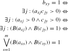

Let us now assume

(11.16)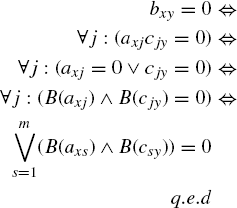

A_a1∨a2 is a sparse matrix with nonzero entries only in the rows and columns of the hyponym and hypernym candidate indices. The matrix A_a1∨a2 can be split up into two components A_{row, a1∨a2} where only the entries in rows index(a1) and index(a2) are nonzero and into the matrix A_{col, a1∨a2} where only the entries in columns index(a1) and index(a2) are nonzero.

The matrix conjunction can then be written as

(11.17)

Similarly, A_{row, a1∨a2} can be further splitted up into

(11.18)

This conjunction contains the nonzero entries for the hyponym and hypernym row (analogously for the columns). The conjunction is given in Figure 11.4, the conjunction in Figure 11.5. The first factor matrix as well as the result of the matrix conjunction are sparse matrices where only the nonzero entries are given in the figures. A_r denotes the rth row vector of matrix A. Usually the hyponym and hypernym nodes are only directly connected to one or two other nodes. Therefore, only a constant number of rows has to be checked for nonzero entries in each step. Thus, with the given intermediate results of with different exponents j, the distance computation can be done in time .

Figure 11.4 Matrix conjunction of A_{hyper/hypo(row)a1∨a2} and where A_{hyper/hypo(row)a1∨a2} is a sparse matrix with nonzero entries only in one row (called: d) and in the two columns p and q.

Figure 11.5 Matrix conjunction of A_{hyper/hypo(col)a1∨a2} and where A_{hyper/hypo(col)a1∨a2} is a sparse matrix with nonzero entries only in one column (called: p) and in the two rows g and h.

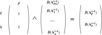
After the distances are calculated, an n × n (n: number of nodes in the product graph) weight matrix W is constructed in the following way:

(11.19)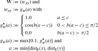

The cosine function is used to realize a smooth transition from 1.0 to 0.1. b, c are fixed positive constants, which can be determined by a parameter optimization (for instance by a grid search). They are currently manually set to b = π/5, c = 2. The application of the weight matrix is done by a component-wise (*) multiplication. Let M₁ and M₂ be two m × n matrices. Then the component-wise product P = M₁ * M₂ with P = (p_xy), M₁ = (m_1,xy), M₂ = (m_2,xy) is defined as p_xy = m_1,xy · m_2,xy for 1 ≤ x ≤ m, 1 ≤ y ≤ n.

An alternative method to derive the weighted matrix, directly determines weights for the edges instead for the nodes. The matrix of distance values for every edge is given by D = (d_xy) with d_xy = i − 1: f_xy = 1 and . The weight matrix W= is then given by . This method also benefits from the proposed matrix decomposition, which speeds up the matrix multiplication enormously. We opted for the first possibility of explicitly deriving distance values for all graph nodes, which allows a more compact representation.

The component-wise multiplication can be done in and is therefore much faster than the ordinary matrix multiplication, which is cubic in runtime. The component-wise multiplication follows the distributive and the commutative laws, which can easily be seen. Thus,

(11.20)

Therefore, the Formula (11.11) changes to

(11.21)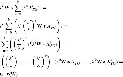

This shows that the transformation method given in Formula (11.11) where the sum is converted from one value of λ to another is still possible.