2.7 Hierarchical Modularity

A high clustering coefficient indicates highly interconnected subnetworks (modules) in real-world networks. However, the next question that arises is regarding the way in which these modules are organized in the network.

Ravasz et al. [25] and Ravasz and Barabási [26] provided an answer for this question by using the degree-dependent clustering coefficient.

This statistical property is defined as

(2.24)

where C_i is the clustering coefficient of node i (see Eq. 2.19).

Ravasz et al. found that the degree-dependent clustering coefficient follows a power–law function in several real-world networks:

(2.25)

where α is a constant and is empirically equal to about 1.

In a random network, the clustering coefficients of all nodes are p, which is independent of the node degree k, because an edge is drawn between a given node pair with the probability p: C^rand(k) = p. Thus, the random network cannot explain this statistical property.

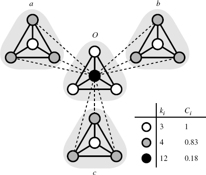
This power–law degree-dependent clustering coefficient indicates that the edge density among neighbors of nodes with a small degree is high and that the edge density among the neighbors of nodes with a large degree is low. In order to explain the relation between this property and the network structure, Ravasz et al. used a simple example, as shown in Figure 2.9.

Figure 2.9 Schematic diagram of the hierarchical modularity. Modules are represented by the triangular-shaded regions. The character near each shaded region corresponds to the name of the module. The solid lines are the edges within a module, and the dashed lines are the edges between modules. The white nodes have 3 edges, and their clustering coefficient is 1. The gray nodes have 4 edges, and their clustering coefficient is 5/6 ≈ 0.83. The black node has 12 edges, and their clustering coefficient is 2/11 ≈ 0.18.

In Figure 2.9, the modules a, b, and c are integrated by the hub (black node) belonging to module O. In this case, the degree of node i (k_i) is proportional to the number of modules to which node i belongs (S_i). The number of edges among the neighbors of node i (M_i) also has a linear relationship with S_i. Thus, we obtain M_i ∝ k_i. Substituting this relation into Equation 2.19, we find the power–law relationship of degree-dependent clustering coefficients C(k) ∝ k⁻¹. Hence, the power–law degree-dependent clustering coefficient reflects hierarchical modularity.

2.7.1 Hierarchical Model

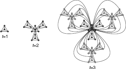
As mentioned above, the network model in Figure 2.9 represents hierarchical modularity. Furthermore, by recursively expanding this network as shown in Figure 2.10, the model network is found to be a scale-free network.

Figure 2.10 Schematic diagram of the hierarchical model with d = 4.

This model network is referred to as the “hierarchical model” [25–27] and is generated by the following procedure. (i) First, we prepare a d-node module (t = 1 in Fig. 2.10) and place its network in G₀. (ii) We generate d − 1 copies of G₀. The peripheral nodes in each copy of G₀ connect to the root. At t = 2 (see Fig. 2.10), for example, d − 1 nodes (excluding the central node) in each module link to the root. (iii) The network generated in Step (ii) is placed in G₀ (i.e., G₀ is updated). The model network expands by repeating Steps (ii) and (iii).

Here, we show that the degree distribution of hierarchical model follows a power law.

From the above procedure, the time evolution of the total number of nodes is d^t. When focusing on the root, the time evolution of the node degree is . By considering this relationship, we find that the model network has d^j nodes with degree (d − 1)[(d − 1)^t−j − 1]/(d − 2) or more, where j is an integer that lies in the range 0 ≤ j ≤ t. Since ln P(≥ k) = ln (d^j/d^t) = (j − t) ln d and ln k ≈ (t − j) ln (d − 1), we directly obtain P(≥ k) = k^{−lnd/ln(d−1)}. Thus, the degree distribution of the hierarchical model is

(2.26)

The hierarchical model network is scale-free and highly clustered. Moreover, it is also a small-world (i.e., L ∝ ln N) network because of its tree structure (see Ref. [28] for details).

2.7.2 Dorogovtsev–Mendes–Samukhin Model

The deterministic models such as the hierarchical model are useful because of their regularity; however, these models also have several limitations. For instance, the number of nodes cannot be closely controlled and the network is relatively artificial. In such a case, probabilistic models are more suitable. The Dorogovtsev–Mendes–Samukhin (DMS) model [29] is a simple probabilistic network model representing scale-free connectivity, hierarchical modularity, and small-world properties.

This model network is generated as follows: (i) a new node is added, and (ii) it is connected to both ends of a randomly selected edge. When an edge drawn between nodes i and j is chosen, for example, the new node k connects to nodes i and j.

This model network becomes scale-free although the preferential attachment mechanism is not directly considered. This is because the random selection of edges is essentially similar to the mechanism of preferential attachment.

We here focus on the time evolution of the degree of node i (k_i). Since the degree of node i increases when an edge leading to the node i is selected, the time evolution is expressed as dk_i/dt = k_i/E, where E is the number of edges and E = 2t. This equation is essentially similar to the BA model, and the degree distribution of the DMS model is P(k) ∝ k⁻³.

Furthermore, the number of edges among the neighbors of node i (M_i) also increases with the degree of node i because one edge leads to node i while the other edges lead to neighbors of node i. Thus, there exists a linear relationship between M_i and k_i. From this relationship, we obtain the power–law degree-dependent clustering coefficient, C(k) ∝ k⁻¹, which indicates hierarchical modularity. Moreover, the DMS mode has a small-world property because it is almost similar to the BA model.