6.5 Comparing Topology Generators
Most past comparisons of topology generators have been limited to the average node degree, the node degree distribution and the joint degree distribution. The rationale for choosing these metrics is that if those properties are closely reproduced then the value of other metrics will also be closely reproduced [33].
In this section, we show that current topology generators are able to match first and second order properties well, that is, average node degree and node degree distribution, but fail to match many other topological metrics. We also discuss the importance of various metrics in our analysis.16
6.5.1 Methodology
For each generator, we specify the required number of nodes and generate 10 topologies of that size to provide confidence intervals for the metrics. We then compute the metrics introduced in Section 6.4 on both the generated and observed AS topologies. All topologies studied in this chapter are undirected, preventing us from considering peering policies and provider–customer relationships. This limitation is forced upon us by the design of the generators as they do not take such policies into account.
Each topology generator uses several parameters, all of which could be tuned to best fit a particular size of topology. However, there are two problems with attempting this tuning. First, doing so requires selecting an appropriate goodness-of-fit measure, of which there are many as noted in Section 6.4. Second, in any case tuning parameters to a particular dataset is of questionable merit since, as we argued in Section 6.1, each dataset is but a sample of reality, having many biases and inaccuracies. Typically, topology generator parameters are tuned to match the number of links in the synthetic and measured networks for a given number of nodes. However, we found this to be infeasible as generating graphs with equal numbers of links from a random model and a power–law model gives completely different outputs. For space reasons, we deal with this particular issue elsewhere [34]; in this chapter, we simply use the default values embedded within each generator.
6.5.2 Topological Metrics
In this section, we discuss the results for each metric separately and analyze the reasons for differences between the observed and the generated topologies.
Table 6.2 displays the values of various metrics (columns) computed for different topologies (rows). Blocks of rows correspond to a single observed topology and the generated topologies with the same number of nodes as the observed topology. Bold numbers represent nearest match of a metric value to that for the relevant observed topology. Rows in each block are ordered with the observed topology first, followed by the generated topologies from oldest to newest generator. For synthetic topologies, the value of the metrics is averaged over the 10 generated instances. Note that Inet requires the number of nodes to be greater than 3037 and hence cannot be compared to the Chinese topology.
Table 6.2 Comparison of AS Level Dataset with Synthetic Topologies.
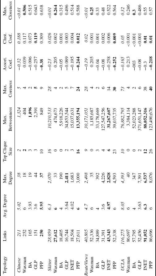
We observe a small but measurable improvement from older to newer generators in some metrics such as maximum degree, maximum coreness, and assortativity coefficient. This suggests that topology generators have successively improved at matching particular properties of the observed topologies. However, the number of links in the generated topologies may differ considerably from the observed topology due to the assumptions made by the generators. The Waxman and BA generators fail to capture the maximum degree, the top clique size, maximum betweenness, and coreness. Those two generators are too simplistic in the assumptions they make about the connectivity of the graphs to generate realistic AS topologies. Waxman relies on a random graph model which cannot capture the clique between tier-1 ASes or the heavy tail of the node degree distribution. BA tries to reproduce the power–law node degrees with its preferential attachment model but fails to reach the maximum node degree, as it only adds edges between new nodes and not between existing ones. Hence, neither of these two models is able to create the highly connected core of tier-1 ASes. PFP and Inet manage to come closer to the values of the metrics of the observed topologies. For Inet this is because it assumes that 30% of the nodes are fully meshed (at the core), whereas for PFP its rich-club connectivity model allows to add edges between existing nodes.
Figure 6.11 displays the CDF of the eigenvalues computed from the normalized Laplacian matrix of each topology.
As with other topological metrics, Inet and PFP perform best. The difference between the topology generators is most easily observed around the eigenvalues equal to 1. These eigenvalues play a special role as they indicate repeated duplications of topological patterns within the network. By duplication, we mean different nodes having the same set of neighbors giving their induced subgraphs the same structure. Through repeated duplication, one can create networks with high multiplicity of eigenvalue 1 [35]. Further, if a network is bipartite, that is, it consists of two connected parts with no links between nodes of the same part, then its spectrum will be symmetric around 1. This phenomenon can also arise through repeated structure duplication.
We observe that the spectra have a high degree of symmetry around the eigenvalue 1, and so the observed AS topologies appear close in spectral terms to a bipartite graph. In the AS topology, many ASes share a similar set of upstream ASes without being directly connected to each other. Inet and PFP are good examples of topology generators where this strategy is implemented. Note that the simple preferential attachment model of BA does not reproduce the eigenvalues around 1 very well. In the simple BA model, new nodes connect randomly to a given number of existing nodes, favoring connections to high degree nodes. In the Internet in contrast, although small ASes may tend to connect to large upstream providers, they might not connect preferentially to the largest ones, connecting instead to national or regional providers. In summary, these results provide further evidence that the interconnection structure of the AS topology is more complex than current models assume.
Figure 6.11 Comparison of cumulative distributions of eigenvalues (from normalized Laplacian).
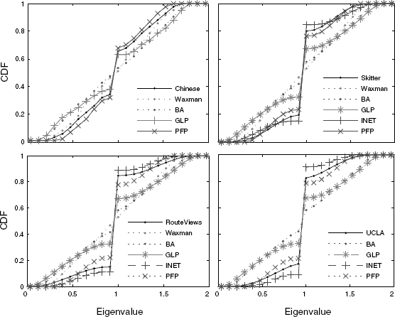
Figure 6.6 Comparison of node degree CCDFs.
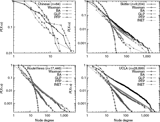
Figure 6.7 Comparison of average neighbor connectivity CCDFs.
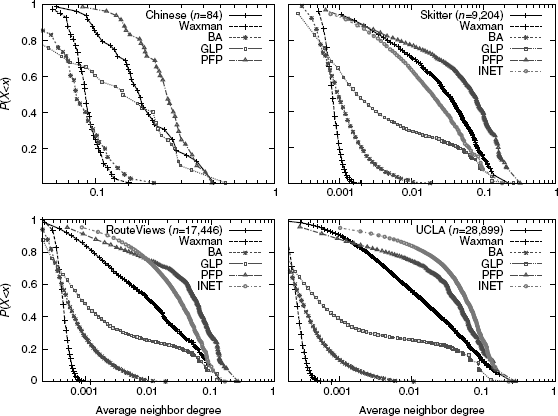
Figure 6.8 Comparison of clustering coefficients.
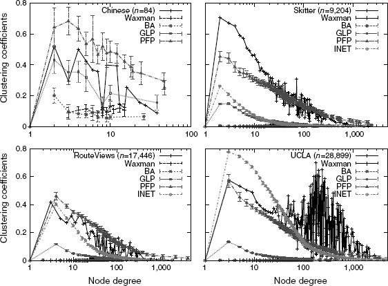
Figure 6.9 Comparison of rich-club connectivity coefficients
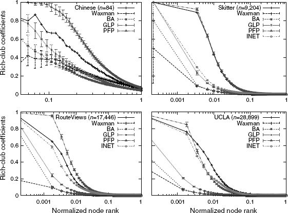
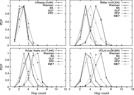
Figure 6.10 Comparison of shortest path distributions (number of hops).
6.5.3 Discussion
Deviations between topology models and observations have been already studied in the literature. However, most works so far have focused on particular topological metrics. Concentrating on particular topological metrics has lead to underestimate the mismatch between the properties of observed AS topologies and what current models produce. When comparing several models with several observed AS topologies as we do, we see that current topology models mostly try to capture some properties of one set of observations from the AS topology. For a topology model to claim to model the Internet's AS topology, we would expect that it tries to approach the properties of observed AS topologies in many respects, which is not the case today.
