5.3 Proofs for Section 4.5 “Measurement of Spectral Correlation –Unknown Support Curves”

In this section, proofs of lemmas and theorems presented in Section 4.5 on bias and covariance of the time-smoothed bifrequency cross-periodogram are reported.

Accounting for the properties of the Fourier transform of a summable function (Champeney 1990) and observing that from Assumption 4.5.2, one obtains

(5.25)

the following result can easily be proved.

Lemma 5.3.1 (Napolitano 2003, Lemma B.1). Under Assumption 4.5.2 (time-smoothing window regularity) and denoting by W_A(f) the Fourier transform of , one obtains that the Fourier transform of the time-smoothing window a_T(t) can be expressed as

(5.26)

with , continuous, and infinitesimal for |f|→ ∞. Moreover, in the sense of distributions, it results that

(5.27)

If is continuous in t = 0, then .

5.3.1 Proof of Lemma 4.5.5 Expected Value of the Time-Smoothed Bifrequency Cross-Periodogram

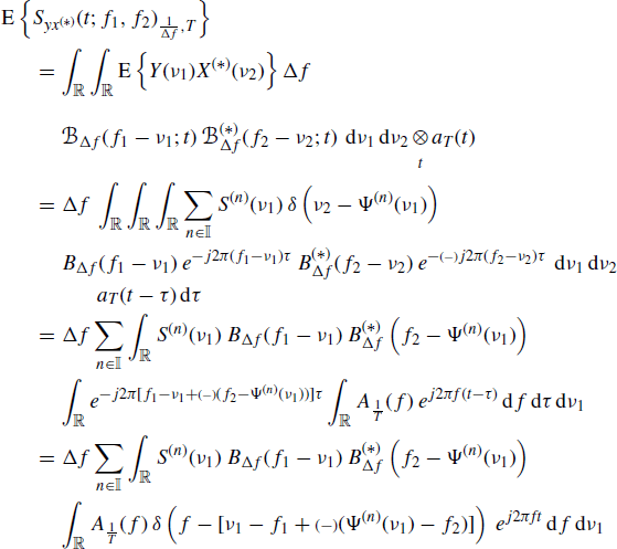
From (4.123) and (5.6), and accounting for (4.15) and (4.107), it follows that

(5.28)

from which, accounting for the sampling property of the Dirac delta, (4.127) immediately follows. In the derivation of (5.28), the formal relationship (Zemanian 1987)

(5.29)

to be intended in the sense of distributions is used.

In the proof, the interchange of expectation, integral, and sum operations can be justified as in the proof of Lemma 4.4.6, accounting for the fact that (Assumption 4.5.2).

5.3.2 Proof of Lemma 4.5.6 Covariance of the Time-Smoothed Bifrequency Cross-Periodogram

It results that (multilinearity property of cumulants (Mendel 1991))

(5.30)

where (4.123) has been accounted for, and the interchange of integral and expectation operations can be justified by the Fubini and Tonelli theorem (Champeney 1990). In fact, by using (4.108) into the right-hand side of (5.30) one has

(5.31)

where

(5.32)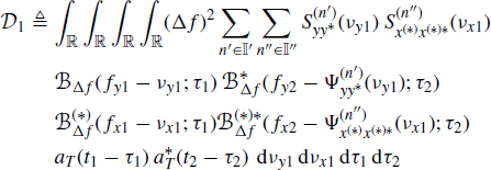

(5.33)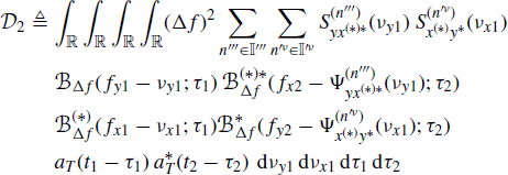

(5.34)

Denoted by D₁(ν_y1, ν_x1, τ₁, τ₂) the integrand function in and accounting for Assumptions 4.4.3a, 4.4.5, and 4.5.2, the result is that

(5.35)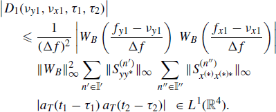

Analogously, it can be shown that the integrand function in is bounded by a summable function. Furthermore, denoted by D₃(ν_y1, ν_x1, ν_y2, τ₁, τ₂) the integrand function in and accounting for Assumptions 4.4.3b, 4.4.5, and 4.5.2, the result is that

(5.36)

By reasoning as for the derivation of (5.28), terms , , and can be shown to be equivalent to , , and , respectively. Then, (4.128) easily follows from (5.30) and (5.31).

Lemma 5.3.2 Let g(f) be a real-valued function of the real variable f, defined in the neighborhood of f = 0. It results that

(5.37)

where δ_f is the Kronecker delta, that is, δ_f = 1 if f = 0 and δ_f = 0 if f ≠ 0.

Proof: Let

(5.38)

We have

(5.39)

if and only if

(5.40)

Since the function δ_u is discontinuous in u = 0, (5.40) is equivalent to

(5.41)

that is, in a neighborhood of Δf = 0. Thus, the limit in (5.39) is 1 if and only if h(Δf) = 1 in a neighborhood of Δf = 0, that is, if and only if g(Δf) = 0 in a neighborhood of Δf = 0.

Note that g(Δf) can be possibly discontinuous or even not defined in Δf = 0. That is, we do not require g(0) = 0.

5.3.3 Proof of Theorem 4.5.7 Asymptotic Expected Value of the Time-Smoothed Bifrequency Cross-Periodogram

By substituting (4.103) and (5.26) into the expression (4.127) of the expected value of the time-smoothed cross-periodogram, and making the variable change λ₁ = (f₁ − ν₁)/Δf one has

(5.42)

Denoted by J_Δf,T(λ₁) the integrand function in (5.42) and accounting for (4.97), Assumption 4.4.5 and Lemma 5.3.1, the result is that

with the right-hand side independent of T and Δf. Thus, the dominated convergence theorem (Champeney 1990) can be applied:

(5.43)

where Lemmas 5.2.1a and 5.2.2 have been accounted for, and the interchange of limit, sum, and integral operations can be justified as in the proof of Lemma 4.4.6.

Since W_A is infinitesimal at ±∞, for any finite Δf the limit for T→ ∞ is zero unless the argument of the inner large parenthesis in the last line of (5.43) is zero. Therefore, accounting for the continuity of W_A(ν), it results in

(5.44)

where is defined in (5.37). To obtain the last equality, observe that, accounting for Lemma 5.3.2, when Δf → 0 the argument of the Kronecker delta in the second line is zero only if f₂ = Ψ⁽ⁿ⁾(f₁) and in a neighborhood of f₁.

Finally, by substituting (5.44) into (5.43), (4.132) is obtained.

5.3.4 Proof of Corollary 4.5.8

At first let us observe that, for Assumption 4.5.3 there is no cluster of support curves and, consequently, for T sufficiently large, it is finite the set of indices n such that, at the fixed point (f₁, f₂), it results |f₂ − Ψ⁽ⁿ⁾(f₁)| T⁻¹. In addition, there exists T₀ > 0 such that for T > T₀ the number of elements of does not change with T.

By considering the Taylor series expansion for Ψ⁽ⁿ⁾(f₁) with second-order Lagrange residual term one has

(5.45)

where , ξ [0, 1]. By substituting (5.45) into

(5.46)

it results in

(5.47)

In Theorem 4.5.7, the asymptotic biasedness of the time-smoothed cross-periodogram is proved for SC processes that are not ACS. This is consequence of the fact that, when in a neighborhood of f₁, the function h⁽ⁿ⁾(λ₁) in (5.42) approaches zero, as T→ ∞ and Δf → 0 with TΔf→ ∞ (see (5.44)). However, if at the point (f₁, f₂) it results that

(5.48)

and

(5.49)

for all i.e., for all n such that

(5.50)

then in substituting (5.47) into (5.42) we can put

(5.51)

In fact, under Assumption 4.4.5 W_B(λ₁) has approximate bandwidth equal to 1, that is, it is significantly different from zero only for λ₁ = O(1) (independently of T and Δf) and W_A(f) is infinitesimal for |f|→ ∞. Thus, by substituting (5.51) into (5.42), for Δf sufficiently small, one obtains (4.136).

Note that (5.48) and (5.49) can be both verified if the second-order derivative of Ψ⁽ⁿ⁾ is bounded (Assumption 4.5.4) and T and Δf are such that TΔf 1 and T(Δf)² 1. If the time-smoothed cross-periodogram is evaluated (with fixed T and Δf) for , with denoting the analysis range, then uniform boundedness in of second-order derivatives is necessary (Assumption 4.5.4).

5.3.5 Proof of Theorem 4.5.9 Asymptotic Covariance of the Time-Smoothed Bifrequency Cross-Periodogram

By substituting (4.103) and (5.26) into (4.129) and making the variable changes λ_y1 = (f_y1 − ν_y1)/Δf and λ_x1 = (f_x1 − ν_x1)/Δf, one obtains

(5.52)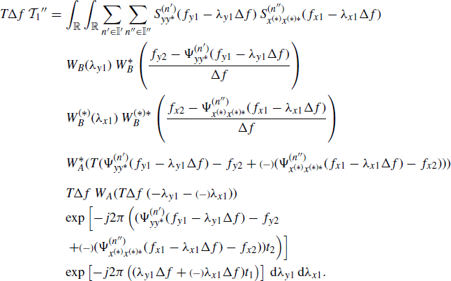

Thus, accounting for Assumption 4.4.3a and Lemma 5.3.1, one has

(5.53)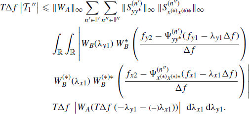

From (5.27) and for , it follows that, in the sense of distributions,

(5.54)

Therefore, for T→ ∞ and Δf → 0 with TΔf→ ∞, accounting for (5.13), (5.54), and the sampling property of Dirac delta, one obtains that with given by (4.138).

Analogously, it can be shown that

(5.55)

with given by (4.139).

Furthermore, by substituting (4.103) and (5.26) into (4.131) and making the variable changes λ_y1 = (f_y1 − ν_y1)/Δf, λ_x1 = (f_x1 − ν_x1)/Δf, and λ_y2 = (f_y2 − ν_y2)/Δf, it results in

(5.56)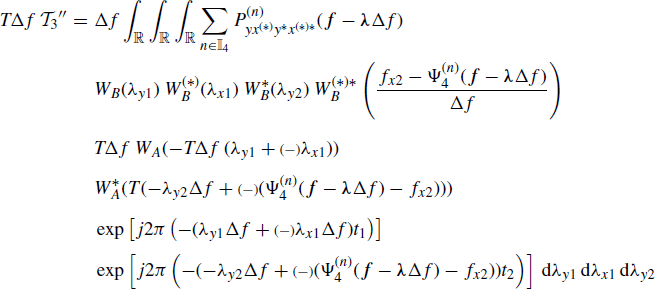

where f − λΔf [f_y1 − λ_y1Δf, f_x1 − λ_x1Δf, f_y2 − λ_y2Δf]. Thus, accounting for Assumptions 4.4.3b and 4.4.5 and Lemma 5.3.1, one has

(5.57)

Accounting for (5.54), one obtains

(5.58)

Therefore, for T→ ∞ and Δf → 0 with TΔf→ ∞,

(5.59)

where the last equality holds under assumption (4.98).

As a final remark, note that the order of the two limits as Δf → 0 and T→ ∞ in Theorems 4.5.7 and 4.5.9 cannot be interchanged. In fact, in the proofs of both Theorems 4.5.7 and 4.5.9 the double limit as Δf → 0 and T→ ∞ is evaluated with TΔf→ ∞ by taking Δf finite and fixed, making T→ ∞ and after making Δf → 0. Analogous results can be obtained if Δf = O(T^−a) with 0 < a < 1. However, the more restrictive condition 1/2 < a < 1 is necessary to assure T(Δf)² → 0 as requested in Corollary 4.5.8 to guarantee (5.49).