Chapter 7

Accounting

Financial analysis spans a variety of accounting applications, including the general ledger, as well as detailed subledgers for purchasing and accounts payable, invoicing and accounts receivable, and fixed assets. Because we've already touched upon purchase orders and invoices earlier in this book, we'll focus on the general ledger in this chapter. Given the need for accurate handling of a company's financial records, general ledgers were one of the first applications to be computerized decades ago. Perhaps some of you are still running your business on a 20-year-old ledger system. In this chapter, we'll discuss the data collected by the general ledger, both in terms of journal entry transactions and snapshots at the close of an accounting period. We'll also talk about the budgeting process.

Chapter 7 discusses the following concepts:

• Bus matrix snippet for accounting processes
• General ledger periodic snapshots and journal transactions
• Chart of accounts
• Period close
• Year-to-date facts
• Multiple fiscal accounting calendars
• Drilling down through a multi-ledger hierarchy
• Budgeting chain and associated processes
• Fixed depth position hierarchies
• Slightly ragged, variable depth hierarchies
• Totally ragged hierarchies of indeterminate depth using a bridge table and alternative modeling techniques
• Shared ownership in a ragged hierarchy
• Time varying ragged hierarchies
• Consolidated fact tables that combine metrics from multiple business processes
• Role of OLAP and packaged analytic financial solutions

Accounting Case Study and Bus Matrix

Because finance was an early adopter of technology, it comes as no surprise that early decision support solutions focused on the analysis of financial data. Financial analysts are some of the most data-literate and spreadsheet-savvy individuals. Often their analysis is disseminated or leveraged by many others in the organization. Managers at all levels need timely access to key financial metrics. In addition to receiving standard reports, they need the ability to analyze performance trends, variances, and anomalies with relative speed and minimal effort. Like many operational source systems, the data in the general ledger is likely scattered among hundreds of tables. Gaining access to financial data and/or creating ad hoc reports may require a decoder ring to navigate through the maze of screens. This runs counter to many organizations' objective to push fiscal responsibility and accountability to the line managers.

The DW/BI system can provide a single source of usable, understandable financial information, ensuring everyone is working off the same data with common definitions and common tools. The audience for financial data is quite diverse in many organizations, ranging from analysts to operational managers to executives. For each group, you need to determine which subset of corporate financial data is needed, in which format, and with what frequency. Analysts and managers want to view information at a high level and then drill to the journal entries for more detail. For executives, financial data from the DW/BI system often feeds their dashboard or scorecard of key performance indicators. Armed with direct access to information, managers can obtain answers to questions more readily than when forced to work through a middleman. Meanwhile, finance can turn their attention to information dissemination and value-added analysis, rather than focusing on report creation.

Improved access to accounting data allows you to focus on opportunities to better manage risk, streamline operations, and identify potential cost savings. Although it has cross-organization impact, many businesses focus their initial DW/BI implementation on strategic, revenue-generating opportunities. Consequently, accounting data is often not the first subject area tackled by the DW/BI team. Given its proficiency with technology, the finance department has often already performed magic with spreadsheets and desktop databases to create workaround analytic solutions, perhaps to its short-term detriment, as these imperfect interim fixes are likely stressed to their limits.

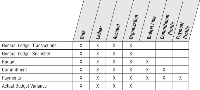
Figure 7.1 illustrates an accounting-focused excerpt from an organization's bus matrix. The dimensions associated with accounting processes, such as the general ledger account or organizational cost center, are frequently used solely by these processes, unlike the core customer, product, and employee dimensions which are used repeatedly across many diverse business processes.

Figure 7.1 Bus matrix rows for accounting processes.

General Ledger Data

The general ledger (G/L) is a core foundation financial system that ties together the detailed information collected by subledgers or separate systems for purchasing, payables (what you owe to others), and receivables (what others owe you). As we work through a basic design for G/L data, you'll discover the need for two complementary schemas with periodic snapshot and transaction fact tables.

General Ledger Periodic Snapshot

We'll begin by delving into a snapshot of the general ledger accounts at the end of each fiscal period (or month if the fiscal accounting periods align with calendar months). Referring back to our four-step process for designing dimensional models (see Chapter 3: Retail Sales), the business process is the general ledger. The grain of this periodic snapshot is one row per accounting period for the most granular level in the general ledger's chart of accounts.

Chart of Accounts

The cornerstone of the general ledger is the chart of accounts. The ledger's chart of accounts is the epitome of an intelligent key because it usually consists of a series of identifiers. For example, the first set of digits may identify the account, account type (for example, asset, liability, equity, income, or expense), and other account rollups. Sometimes intelligence is embedded in the account numbering scheme. For example, account numbers from 1,000 through 1,999 might be asset accounts, whereas account numbers ranging from 2,000 to 2,999 may identify liabilities. Obviously, in the data warehouse, you'd include the account type as a dimension attribute rather than forcing users to filter on the first digit of the account number.

The chart of accounts likely associates the organization cost center with the account. Typically, the organization attributes provide a complete rollup from cost center to department to division, for example. If the corporate general ledger combines data across multiple business units, the chart of accounts would also indicate the business unit or subsidiary company.

Obviously, charts of accounts vary from organization to organization. They're often extremely complicated, with hundreds or even thousands of cost centers in large organizations. In this case study vignette, the chart of accounts naturally decomposes into two dimensions. One dimension represents accounts in the general ledger, whereas the other represents the organization rollup.

The organization rollup may be a fixed depth hierarchy, which would be handled as separate hierarchical attributes in the cost center dimension. If the organization hierarchy is ragged with an unbalanced rollup structure, you need the more powerful variable depth hierarchy techniques described in the section “Ragged Variable Depth Hierarchies.”

If you are tasked with building a comprehensive general ledger spanning multiple organizations in the DW/BI system, you should try to conform the chart of accounts so the account types mean the same thing across organizations. At the data level, this means the master conformed account dimension contains carefully defined account names. Capital Expenditures and Office Supplies need to have the same financial meaning across organizations. Of course, this kind of conformed dimension has an old and familiar name in financial circles: the uniform chart of accounts.

The G/L sometimes tracks financial results for multiple sets of books or subledgers to support different requirements, such as taxation or regulatory agency reporting. You can treat this as a separate dimension because it's such a fundamental filter, but we alert you to carefully read the cautionary note in the next section.

Period Close

At the end of each accounting period, the finance organization is responsible for finalizing the financial results so that they can be officially reported internally and externally. It typically takes several days at the end of each period to reconcile and balance the books before they can be closed with finance's official stamp of approval. From there, finance's focus turns to reporting and interpreting the results. It often produces countless reports and responds to countless variations on the same questions each month.

Financial analysts are constantly looking to streamline the processes for period-end closing, reconciliation, and reporting of general ledger results. Although operational general ledger systems often support these requisite capabilities, they may be cumbersome, especially if you're not dealing with a modern G/L. This chapter focuses on easily analyzing the closed financial results, rather than facilitating the close. However, in many organizations, general ledger trial balances are loaded into the DW/BI system leveraging the capabilities of the DW/BI presentation area to find the needles in the general ledger haystack, and then making the appropriate operational adjustments before the period ends.

The sample schema in Figure 7.2 shows general ledger account balances at the end of each accounting period which would be very useful for many kinds of financial analyses, such as account rankings, trending patterns, and period-to-period comparisons.

Figure 7.2 General ledger periodic snapshot.

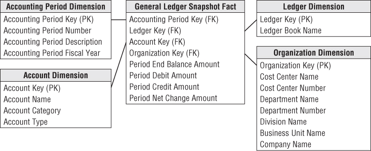
For the moment, we're just representing actual ledger facts in the Figure 7.2 schema; we'll expand our view to cover budget data in the section “Budgeting Process.” In this table, the balance amount is a semi-additive fact. Although the balance doesn't represent G/L activity, we include the fact in the design because it is so useful. Otherwise, you would need to go back to the beginning of time to calculate an accurate end-of-period balance.

The two most important dimensions in the proposed general ledger design are account and organization. The account dimension is carefully derived from the uniform chart of accounts in the enterprise. The organization dimension describes the financial reporting entities in the enterprise. Unfortunately, these two crucial dimensions almost never conform to operational dimensions such as customer, product, service, or facility. This leads to a characteristic but unavoidable business user frustration that the “GL doesn't tie to my operational reports.” It is best to gently explain this to the business users in the interview process, rather than promising to fix it because this is a deep seated issue in the underlying data.

Year-to-Date Facts

Designers are often tempted to store “to-date” columns in fact tables. They think it would be helpful to store quarter-to-date or year-to-date additive totals on each fact row so they don't need to calculate them. Remember that numeric facts must be consistent with the grain. To-date facts are not true to the grain and are fraught with peril. When fact rows are queried and summarized in arbitrary ways, these untrue-to-the-grain facts produce nonsensical, overstated results. They should be left out of the relational schema design and calculated in the BI reporting application instead. It's worth noting that OLAP cubes handle to-date metrics more gracefully.

Multiple Currencies Revisited

If the general ledger consolidates data that has been captured in multiple currencies, you would handle it much as we discussed in Chapter 6: Order Management. With financial data, you typically want to represent the facts both in terms of the local currency, as well as a standardized corporate currency. In this case, each fact table row would represent one set of fact amounts expressed in local currency and a separate set of fact amounts on the same row expressed in the equivalent corporate currency. Doing so allows you to easily summarize the facts in a common corporate currency without jumping through hoops in the BI applications. Of course, you'd also add a currency dimension as a foreign key in the fact table to identify the local currency type.

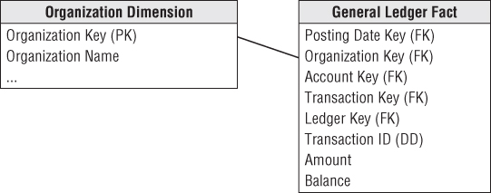
General Ledger Journal Transactions

While the end-of-period snapshot addresses a multitude of financial analyses, many users need to dive into the underlying details. If an anomaly is identified at the summary level, analysts want to look at the detailed transactions to sort through the issue. Others need access to the details because the summarized monthly balances may obscure large disparities at the granular transaction level. Again, you can complement the periodic snapshot with a detailed journal entry transaction schema. Of course, the accounts payable and receivable subledgers may contain transactions at progressively lower levels of detail, which would be captured in separate fact tables with additional dimensionality.

The grain of the fact table is now one row for every general ledger journal entry transaction. The journal entry transaction identifies the G/L account and the applicable debit or credit amount. As illustrated in Figure 7.3, several dimensions from the last schema are reused, including the account and organization. If the ledger tracks multiple sets of books, you'd also include the ledger/book dimension. You would normally capture journal entry transactions by transaction posting date, so use a daily-grained date table in this schema. Depending on the business rules associated with the source data, you may need a second role-playing date dimension to distinguish the posting date from the effective accounting date.

Figure 7.3 General ledger journal entry transactions.

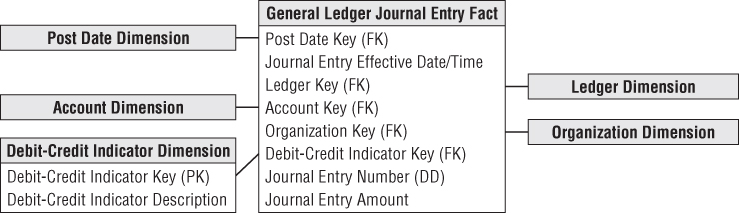
The journal entry number is likely a degenerate dimension with no linkage to an associated dimension table. If the journal entry numbers from the source are ordered, then this degenerate dimension can be used to order the journal entries because the calendar date dimension on this fact table is too coarse to provide this sorting. If the journal entry numbers do not easily support the sort, then an effective date/time stamp must be added to the fact table. Depending on the source data, you may have a journal entry transaction type and even a description. In this situation, you would create a separate journal entry transaction profile dimension (not shown). Assuming the descriptions are not just freeform text, this dimension would have significantly fewer rows than the fact table, which would have one row per journal entry line. The specific journal entry number would still be treated as degenerate.

Each row in the journal entry fact table is identified as either a credit or a debit. The debit/credit indicator takes on two, and only two, values.

Multiple Fiscal Accounting Calendars

In Figure 7.3, the data is captured by posting date, but users may also want to summarize the data by fiscal account period. Unfortunately, fiscal accounting periods often do not align with standard Gregorian calendar months. For example, a company may have 13 4-week accounting periods in a fiscal year that begins on September 1 rather than 12 monthly periods beginning on January 1. If you deal with a single fiscal calendar, then each day in a year corresponds to a single calendar month, as well as a single accounting period. Given these relationships, the calendar and accounting periods are merely hierarchical attributes on the daily date dimension. The daily date dimension table would simultaneously conform to a calendar month dimension table, as well as to a fiscal accounting period dimension table.

In other situations, you may deal with multiple fiscal accounting calendars that vary by subsidiary or line of business. If the number of unique fiscal calendars is a fixed, low number, then you can include each set of uniquely labeled fiscal calendar attributes on a single date dimension. A given row in the daily date dimension would be identified as belonging to accounting period 1 for subsidiary A but accounting period 7 for subsidiary B.

In a more complex situation with a large number of different fiscal calendars, you could identify the official corporate fiscal calendar in the date dimension. You then have several options to address the subsidiary-specific fiscal calendars. The most common approach is to create a date dimension outrigger with a multipart key consisting of the date and subsidiary keys. There would be one row in this table for each day for each subsidiary. The attributes in this outrigger would consist of fiscal groupings (such as fiscal week end date and fiscal period end date). You would need a mechanism for filtering on a specific subsidiary in the outrigger. Doing so through a view would then allow the outrigger to be presented as if it were logically part of the date dimension table.

A second approach for tackling the subsidiary-specific calendars would be to create separate physical date dimensions for each subsidiary calendar, using a common set of surrogate date keys. This option would likely be used if the fact data were decentralized by subsidiary. Depending on the BI tool's capabilities, it may be easier to either filter on the subsidiary outrigger as described in option 1 or ensure usage of the appropriate subsidiary-specific physical date dimension table (option 2). Finally, you could allocate another foreign key in the fact table to a subsidiary fiscal period dimension table. The number of rows in this table would be the number of fiscal periods (approximately 36 for 3 years) times the number of unique calendars. This approach simplifies user access but puts additional strain on the ETL system because it must insert the appropriate fiscal period key during the transformation process.

Drilling Down Through a Multilevel Hierarchy

Very large enterprises or government agencies may have multiple ledgers arranged in an ascending hierarchy, perhaps by enterprise, division, and department. At the lowest level, department ledger entries may be consolidated to roll up to a single division ledger entry. Then the division ledger entries may be consolidated to the enterprise level. This would be particularly common for the periodic snapshot grain of these ledgers. One way to model this hierarchy is by introducing the parent snapshot's fact table surrogate key in the fact table, as shown in Figure 7.4. In this case, because you define a parent/child relationship between rows, you add an explicit fact table surrogate key, a single column numeric identifier incremented as you add rows to the fact table.

Figure 7.4 Design for drilling down through multiple ledgers.

You can use the parent snapshot surrogate key to drill down in your multilayer general ledger. Suppose that you detect a large travel amount at the top level of the ledger. You grab the surrogate key for that high-level entry and then fetch all the entries whose parent snapshot key equals that key. This exposes the entries at the next lower level that contribute to the original high-level record of interest. The SQL would look something like this:

Select * from GL_Fact where Parent_Snapshot_key =
  (select fact_table_surrogate_key from GL_Fact f, Account a
   where <joins> and a.Account = 'Travel' and f.Amount > 1000)

Financial Statements

One of the primary functions of a general ledger system is to produce the organization's official financial reports, such as the balance sheet and income statement. The operational system typically handles the production of these reports. You wouldn't want the DW/BI system to attempt to replace the reports published by the operational financial systems.

However, DW/BI teams sometimes create complementary aggregated data that provides simplified access to report information that can be more widely disseminated throughout the organization. Dimensions in the financial statement schema would include the accounting period and cost center. Rather than looking at general ledger account level data, the fact data would be aggregated and tagged with the appropriate financial statement line number and label. In this manner, managers could easily look at performance trends for a given line in the financial statement over time for their organization. Similarly, key performance indicators and financial ratios may be made available at the same level of detail.

Budgeting Process

Most modern general ledger systems include the capability to integrate budget data into the general ledger. However, if the G/L either lacks this capability or it has not been implemented, you need to provide an alternative mechanism for supporting the budgeting process and variance comparisons.

Within most organizations, the budgeting process can be viewed as a series of events. Prior to the start of a fiscal year, each cost center manager typically creates a budget, broken down by budget line items, which is then approved. In reality, budgeting is seldom simply a once-per-year event. Budgets are becoming more dynamic because there are budget adjustments as the year progresses, reflecting changes in business conditions or the realities of actual spending versus the original budget. Managers want to see the current budget's status, as well as how the budget has been altered since the first approved version. As the year unfolds, commitments to spend the budgeted monies are made. Finally, payments are processed.

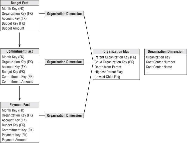
As a dimensional modeler, you can view the budgeting chain as a series of fact tables, as shown in Figure 7.5. This chain consists of a budget fact table, commitments fact table, and payments fact table, where there is a logical flow that starts with a budget being established for each organization and each account. Then during the operational period, commitments are made against the budgets, and finally payments are made against those commitments.

Figure 7.5 Chain of budget processes.

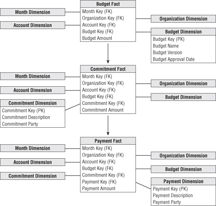
We'll begin with the budget fact table. For an expense budget line item, each row identifies what an organization in the company is allowed to spend for what purpose during a given time frame. Similarly, if the line item reflects an income forecast, which is just another variation of a budget, it would identify what an organization intends to earn from what source during a time frame.

You could further identify the grain to be a snapshot of the current status of each line item in each budget each month. Although this grain has a familiar ring to it (because it feels like a management report), it is a poor choice as the fact table grain. The facts in such a “status report” are all semi-additive balances, rather than fully additive facts. Also, this grain makes it difficult to determine how much has changed since the previous month or quarter because you must obtain the rows from several time periods and then subtract them from each other. Finally, this grain choice would require the fact table to contain many duplicated rows when nothing changes in successive months for a given line item.

Instead, the grain you're interested in is the net change of the budget line item in an organizational cost center that occurred during the month. Although this suffices for budget reporting purposes, the accountants eventually need to tie the budget line item back to a specific general ledger account that's affected, so you'll also go down to the G/L account level.

Given the grain, the associated budget dimensions would include effective month, organization cost center, budget line item, and G/L account, as illustrated in Figure 7.6. The organization is identical to the dimension used earlier with the general ledger data. The account dimension is also a reused dimension. The only complication regarding the account dimension is that sometimes a single budget line item impacts more than one G/L account. In that case, you would need to allocate the budget line to the individual G/L accounts. Because the grain of the budget fact table is by G/L account, a single budget line for a cost center may be represented as several rows in the fact table.

Figure 7.6 Budget schema.

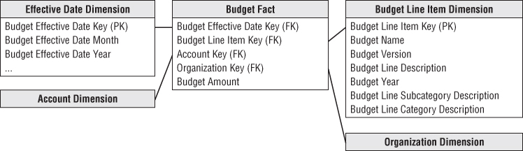
The budget line item identifies the purpose of the proposed spending, such as employee wages or office supplies. There are typically several levels of summarization categories associated with a budget line item. All the budget line items may not have the same number of levels in their summarization hierarchy, such as when some only have a category rollup, but not a subcategory. In this case, you may populate the dimension attributes by replicating the category name in the subcategory column to avoid having line items roll up to a Not Applicable subcategory bucket. The budget line item dimension would also identify the budget year and/or budget version.

The effective month is the month during which the budget changes are posted. The first entries for a given budget year would show the effective month when the budget is first approved. If the budget is updated or modified as the budget year gets underway, the effective months would occur during the budget year. If you don't adjust a budget throughout the year, then the only entries would be the first ones when the budget is initially approved. This is what is meant when the grain is specified to be the net change. It's critical that you understand this point, or you won't understand what is in this budget fact table or how it's used.

Sometimes budgets are created as annual spending plans; other times, they're broken down by month or quarter. Figure 7.6 assumes the budget is an annual amount, with the budget year identified in the budget line item dimension. If you need to express the budget data by spending month, you would need to include a second month dimension table that plays the role of spending month.

The budget fact table has a single budget amount fact that is fully additive. If you budget for a multinational organization, the budget amount may be tagged with the expected currency conversion factor for planning purposes. If the budget amount for a given budget line and account is modified during the year, an additional row is added to the budget fact table representing the net change. For example, if the original budget were $200,000, you might have another row in June for a $40,000 increase and then another in October for a negative $25,000 as you tighten your belt going into year-end.

When the budget year begins, managers make commitments to spend the budget through purchase orders, work orders, or other forms of contracts. Managers are keenly interested in monitoring their commitments and comparing them to the annual budget to manage their spending. We can envision a second fact table for the commitments (refer to Figure 7.5) that shares the same dimensions, in addition to dimensions identifying the specific commitment document (purchase order, work order, or contract) and commitment party. In this case, the fact would be the committed amount.

Finally, payments are made as monies are transferred to the party named in the commitment. From a practical point of view, the money is no longer available in the budget when the commitment is made. But the finance department is interested in the relationship between commitments and payments because it manages the company's cash. The dimensions associated with the payments fact table would include the commitment fact table dimensions, plus a payment dimension to identify the type of payment, as well as the payee to whom the payment was actually made. Referring the budgeting chain shown in Figure 7.5, the list of dimensions expands as you move from the budget to commitments to payments.

With this design, you can create a number of interesting analyses. To look at the current budgeted amount by department and line item, you can constrain on all dates up to the present, adding the amounts by department and line item. Because the grain is the net change of the line items, adding up all the entries over time does exactly the right thing. You end up with the current approved budget amount, and you get exactly those line items in the given departments that have a budget.

To ask for all the changes to the budget for various line items, simply constrain on a single month. You'll report only those line items that experienced a change during the month.

To compare current commitments to the current budget, separately sum the commitment amounts and budget amounts from the beginning of time to the current date (or any date of interest). Then combine the two answer sets on the row headers. This is a standard drill-across application using multipass SQL. Similarly, you could drill across commitments and payments.

Dimension Attribute Hierarchies

Although the budget chain use case described in this chapter is reasonably simple, it contains a number of hierarchies, along with a number of choices for the designer. Remember a hierarchy is defined by a series of many-to-one relationships. You likely have at least four hierarchies: calendar levels, account levels, geographic levels, and organization levels.

Fixed Depth Positional Hierarchies

In the budget chain, the calendar levels are familiar fixed depth position hierarchies. As the name suggests, a fixed position hierarchy has a fixed set of levels, all with meaningful labels. Think of these levels as rollups. One calendar hierarchy may be day ⇒ fiscal period ⇒ year. Another could be day ⇒ month ⇒ year. These two hierarchies may be different if there is no simple relationship between fiscal periods and months. For example, some organizations have 5-4-4 fiscal periods, consisting of a 5-week span followed by two 4-week spans. A single calendar date dimension can comfortably represent these two hierarches at the same time in sets of parallel attributes since the grain of the date dimension is the individual day.

The account dimension may also have a fixed many-to-one hierarchy such as executive level, director level, and manager level accounts. The grain of the dimension is the manager level account, but the detailed accounts at the lowest grain roll up to the director and executive levels.

In a fixed position hierarchy, it is important that each level have a specific name. That way the business user knows how to constrain and interpret each level.

Slightly Ragged Variable Depth Hierarchies

Geographic hierarchies present an interesting challenge. Figure 7.7 shows three possibilities. The simple location has four levels: address, city, state, and country. The medium complex location adds a zone level, and the complex location adds both district and zone levels. If you need to represent all three types of locations in a single geographic hierarchy, you have a slightly variable hierarchy. You can combine all three types if you are willing to make a compromise. For the medium location that has no concept of district, you can propagate the city name down into the district attribute. For the simple location that has no concept of either district or zone, you can propagate the city name down into both these attributes. The business data governance representatives may instead decide to propagate labels upward or even populate the empty levels with Not Applicable. The business representatives need to visualize the appropriate row label values on a report if the attribute is grouped on. Regardless of the business rules applied, you have the advantage of a clean positional design with attribute names that make reasonable sense across all three geographies. The key to this compromise is the narrow range of geographic hierarchies, ranging from four levels to only six levels. If the data ranged from four levels to eight or ten or even more, this design compromise would not work. Remember the attribute names need to make sense.

Figure 7.7 Sample data values exist simultaneously in a single location dimension containing simple, intermediate, and complex hierarchies.

Ragged Variable Depth Hierarchies

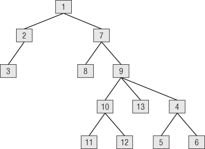
In the budget use case, the organization structure is an excellent example of a ragged hierarchy of indeterminate depth. In this chapter, we often refer to the hierarchical structure as a “tree” and the individual organizations in that tree as “nodes.” Imagine your enterprise consists of 13 organizations with the rollup structure shown in Figure 7.8. Each of these organizations has its own budget, commitments, and payments.

Figure 7.8 Organization rollup structure.

For a single organization, you can request a specific budget for an account with a simple join from the organization dimension to the fact table, as shown in Figure 7.9. But you also want to roll up the budget across portions of the tree or even all the tree. Figure 7.9 contains no information about the organizational rollup.

Figure 7.9 Organization dimension joined to fact table.

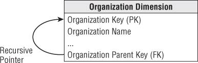
The classic way to represent a parent/child tree structure is by placing recursive pointers in the organization dimension from each row to its parent, as shown in Figure 7.10. The original definition of SQL did not provide a way to evaluate these recursive pointers. Oracle implemented a CONNECT BY function that traversed these pointers in a downward fashion starting at a high-level parent in the tree and progressively enumerated all the child nodes in lower levels until the tree was exhausted. But the problem with Oracle CONNECT BY and other more general approaches, such as SQL Server's recursive common table expressions, is that the representation of the tree is entangled with the organization dimension because these approaches depend on the recursive pointer embedded in the data. It is impractical to switch from one rollup structure to another because many of the recursive pointers would have to be destructively modified. It is also impractical to maintain organizations as type 2 slowly changing dimension attributes because changing the key for a high-level node would ripple key changes down to the bottom of the tree.

Figure 7.10 Classic parent/child recursive design.

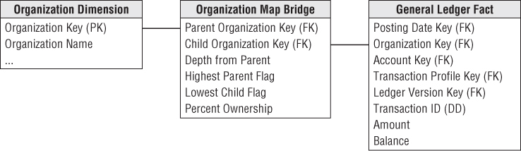
The solution to the problem of representing arbitrary rollup structures is to build a special kind of bridge table that is independent from the primary dimension table and contains all the information about the rollup. The grain of this bridge table is each path in the tree from a parent to all the children below that parent, as shown in Figure 7.11. The first column in the map table is the primary key of the parent, and the second column is the primary key of the child. A row must be constructed from each possible parent to each possible child, including a row that connects the parent to itself.

Figure 7.11 Organization map bridge table sample rows.

The example tree depicted in Figure 7.8 results in 43 rows in Figure 7.11. There are 13 paths from node number 1, 5 paths from node number 2, one path from node number 3 to itself, as so on.

The highest parent flag in the map table means the particular path comes from the highest parent in the tree. The lowest child flag means the particular path ends in a “leaf node” of the tree.

If you constrain the organization dimension table to a single row, you can join the dimension table to the map table to the fact table, as shown in Figure 7.12. For example, if you constrain the organization table to node number 1 and simply fetch an additive fact from the fact table, you get 13 hits on the fact table, which traverses the entire tree in a single query. If you perform the same query except constrain the map table lowest child flag to true, then you fetch only the additive fact from the six leaf nodes, numbers 3, 5, 6, 8, 10, and 11. Again, this answer was computed without traversing the tree at query time!

Figure 7.12 Joining organization map bridge table to fact table.

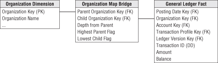
You must be careful when using the map bridge table to constrain the organization dimension to a single row, or else you risk overcounting the children and grandchildren in the tree. For example, if instead of a constraint such as “Node Organization Number = 1” you constrain on “Node Organization Location = California”, you would have this problem. In this case you need to craft a custom query, rather than a simple join, with the following constraint:

GLfact.orgkey in (select distinct bridge.childkey
              from innerorgdim, bridge
              where innerorgdim.state = 'California' and
              innerorgdim.orgkey = bridge.parentkey)

Shared Ownership in a Ragged Hierarchy

The map table can represent partial or shared ownership, as shown in Figure 7.13. For instance, suppose node 10 is 50 percent owned by node 6 and 50 percent owned by node 11. In this case, any budget or commitment or payment attributed to node 10 flows upward through node 6 with a 50 percent weighting and also upward through node 11 with a 50 percent weighting. You now need to add extra path rows to the original 43 rows to accommodate the connection of node 10 up to node 6 and its parents. All the relevant path rows ending in node 10 now need a 50 percent weighting in the ownership percentage column in the map table. Other path rows not ending in node 10 do not have their ownership percentage column changed.

Figure 7.13 Bridge table for ragged hierarchy with shared ownership.

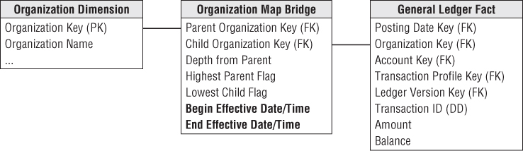
Time Varying Ragged Hierarchies

The ragged hierarchy bridge table can accommodate slowly changing hierarchies with the addition of two date/time stamps, as shown in Figure 7.14. When a given node no longer is a child of another node, the end effective date/time of the old relationship must be set to the date/time of the change, and new path rows inserted into the bridge table with the correct begin effective date/time.

Figure 7.14 Bridge table for time varying ragged hierarchies.

Modifying Ragged Hierarchies

The organization map bridge table can easily be modified. Suppose you want to move nodes 4, 5, and 6 from their original location reporting up to node 2 to a new location reporting up to node 9, as shown in Figure 7.15.

Figure 7.15 Changes to Figure 7.8's organization structure.

In the static case in which the bridge table only reflects the current rollup structure, you merely delete the higher level paths in the tree pointing into the group of nodes 4, 5, and 6. Then you attach nodes 4, 5, and 6 into the parents 1, 7, and 9. Here is the static SQL:

Delete from Org_Map where child_org in (4, 5,6) and
  parent_org not in (4,5,6)
Insert into Org_Map (parent_org, child_org)
  select parent_org, 4 from Org_Map where parent_org in (1, 7, 9)
Insert into Org_Map (parent_org, child_org)
  select parent_org, 5 from Org_Map where parent_org in (1, 7, 9)
Insert into Org_Map (parent_org, child_org)
  select parent_org, 6 from Org_Map where parent_org in (1, 7, 9)

In the time varying case in which the bridge table has the pair of date/time stamps, the logic is similar. You can find the higher level paths in the tree pointing into the group of nodes 4, 5, and 6 and set their end effective date/times to the moment of the change. Then you attach nodes 4, 5, and 6 into the parents 1, 7, and 9 with the appropriate date/times. Here is the time varying SQL:

Update Org_Map set end_eff_date = #December 31, 2012#
  where child_org in (4, 5,6) and parent_org not in (4,5,6)
  and #Jan 1, 2013# between begin_eff_date and end_eff_date
Insert into Org_Map
  (parent_org, child_org, begin_eff_date, end_eff_date)
  values (1, 4, #Jan 1, 2013#, #Dec 31, 9999#)
Insert into Org_Map
  (parent_org, child_org, begin_eff_date, end_eff_date)
  values (7, 4, #Jan 1, 2013#, #Dec 31, 9999#)
Insert into Org_Map
  (parent_org, child_org, begin_eff_date, end_eff_date)
  values (9, 4, #Jan 1, 2013#, #Dec 31, 9999#)
Identical insert statements for nodes 5 and 6 …

This simple recipe for changing the bridge table avoids nightmarish scenarios when changing other types of hierarchical models. In the bridge table, only the paths directly involved in the change are affected. All other paths are untouched. In most other schemes with clever node labels, a change in the tree structure can affect many or even all the nodes in the tree, as shown in the next section.

Alternative Ragged Hierarchy Modeling Approaches

In addition to using recursive pointers in the organization dimension, there are at least two other ways to model a ragged hierarchy, both involving clever columns placed in the organization dimension. There are two disadvantages to these schemes compared to the bridge table approach. First, the definition of the hierarchy is locked into the dimension and cannot easily be replaced. Second, both of these schemes are vulnerable to a relabeling disaster in which a large part of the tree must be relabeled due to a single small change. Textbooks (like this one!) usually show a tiny example, but you need to tread cautiously if there are thousands of nodes in your tree.

One scheme adds a pathstring attribute to the organization dimension table, as shown in Figure 7.16. The values of the pathstring attribute are shown within each node. In this scenario, there is no bridge table. At each level, the pathstring starts with the full pathstring of the parent and then adds the letters A, B, C, and so on, from left to right under that parent. The final character is a “+” if the node has children and is a period if the node has no children. The tree can be navigated by using wild cards in constraints against the pathstring, for example,

• A* retrieves the whole tree where the asterisk is a variable length wild card.
• *. retrieves only the leaf nodes.
• ?+ retrieves the topmost node where the question mark is a single character wild card.

Figure 7.16 Alternate ragged hierarchy design using pathstring attribute.

The pathstring approach is fairly sensitive to relabeling ripples caused by organization changes; if a new node is inserted somewhere in the tree, all the nodes to the right of that node under the same parent must be relabeled.

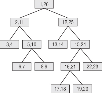
Another similar scheme, known to computer scientists as the modified preordered tree traversal approach, numbers the tree as shown in Figure 7.17. Every node has a pair of numbers that identifies all the nodes below that point. The whole tree can be enumerated by using the node numbers in the topmost node. If the values in each node have the names Left and Right, then all the nodes in the example tree can be found with the constraint “Left between 1 and 26.” Leaf nodes can be found where Left and Right differ by 1, meaning there aren't any children. This approach is even more vulnerable to the relabeling disaster than the pathstring approach because the entire tree must be carefully numbered in sequence, top to bottom and left to right. Any change to the tree causes the entire rest of the tree to the right to be relabeled.

Figure 7.17 Alternative ragged hierarchy design using the modified preordered tree traversal approach.

Advantages of the Bridge Table Approach for Ragged Hierarchies

Although the bridge table requires more ETL work to set up and more work when querying, it offers exceptional flexibility for analyzing ragged hierarches of indeterminate depth. In particular, the bridge table allows

• Alternative rollup structures to be selected at query time
• Shared ownership rollups
• Time varying ragged hierarchies
• Limited impact when nodes undergo slowly changing dimension (SCD) type 2 changes
• Limited impact when the tree structure is changed

You can use the organization hierarchy bridge table to fetch a fact across all three fact tables in the budget chain. Figure 7.18 shows how an organization map table can connect to the three budget chain fact tables. This would allow a drill-across report such as finding all the travel budgets, commitments, and payments made by all the lowest leaf nodes in a complex organizational structure.

Figure 7.18 Drilling across and rolling up the budget chain.

Consolidated Fact Tables

In the last section, we discussed comparing metrics generated by separate business processes by drilling across fact tables, such as budget and commitments. If this type of drill-across analysis is extremely common in the user community, it likely makes sense to create a single fact table that combines the metrics once rather than relying on business users or their BI reporting applications to stitch together result sets, especially given the inherent issues of complexity, accuracy, tool capabilities, and performance.

Most typically, business managers are interested in comparing actual to budget variances. At this point, you can presume the annual budgets and/or forecasts have been broken down by accounting period. Figure 7.19 shows the actual and budget amounts, as well as the variance (which is a calculated difference) by the common dimensions.

Figure 7.19 Actual versus budget consolidated fact table.

Again, in a multinational organization, you would likely see the actual amounts in both local and the equivalent standard currency, based on the effective conversion rate. In addition, you may convert the actual results based on the planned currency conversion factor. Given the unpredictable nature of currency fluctuations, it is useful to monitor performance based on both the effective and planned conversion rates. In this manner, remote managers aren't penalized for currency rate changes outside their control. Likewise, finance can better understand the big picture impact of unexpected currency conversion fluctuations on the organization's annual plan.

Fact tables that combine metrics from multiple business processes at a common granularity are referred to as consolidated fact tables. Although consolidated fact tables can be useful, both in terms of performance and usability, they often represent a dimensionality compromise as they consolidate facts at the “least common denominator” of dimensionality. One potential risk associated with consolidated fact tables is that project teams sometimes base designs solely on the granularity of the consolidated table, while failing to meet user requirements that demand the ability to dive into more granular data. These schemas run into serious problems if project teams attempt to force a one-to-one correspondence to combine data with different granularity or dimensionality.

Role of OLAP and Packaged Analytic Solutions

While discussing financial dimensional models in the context of relational databases, it is worth noting that multidimensional OLAP vendors have long played a role in this arena. OLAP products have been used extensively for financial reporting, budgeting, and consolidation applications. Relational dimensional models often feed financial OLAP cubes. OLAP cubes can deliver fast query performance that is critical for executive usage. The data volumes, especially for general ledger balances or financial statement aggregates, do not typically overwhelm the practical size constraints of a multidimensional product. OLAP is well suited to handle complicated organizational rollups, as well as complex calculations, including inter-row manipulations. Most OLAP vendors provide finance-specific capabilities, such as financial functions (for example, net present value or compound growth), the appropriate handling of financial statement data (in the expected sequential order such as income before expenses), and the proper treatment of debits and credits depending on the account type, as well as more advanced functions such as financial consolidation. OLAP cubes often also readily support complex security models, such as limiting access to detailed data while providing more open access to summary metrics.

Given the standard nature of general ledger processing, purchasing a general ledger package rather than attempting to build one from scratch has been a popular route for years. Nearly all the operational packages also offer a complementary analytic solution, sometimes in partnership with an OLAP vendor. In many cases, precanned solutions based on the vendor's cumulative experience are a sound way to jump start a financial DW/BI implementation with potentially reduced cost and risk. The analytic solutions often have tools to assist with the extraction and staging of the operational data, as well as tools to assist with analysis and interpretation. However, when leveraging packaged solutions, you need to be cautious in order to avoid stovepipe applications. You could easily end up with separate financial, CRM, human resources, and ERP packaged analytic solutions from as many different vendors, none of which integrate with other internal data. You need to conform dimensions across the entire DW/BI environment, regardless of whether you build a solution or implement packages. Packaged analytic solutions can turbocharge a DW/BI implementation; however, they do not alleviate the need for conformance. Most organizations inevitably rely on a combination of building, buying, and integrating for a complete solution.

Summary

In this chapter, we focused primarily on financial data in the general ledger, both in terms of periodic snapshots as well as journal entry transactions. We discussed the handling of common G/L data challenges, including multiple currencies, multiple fiscal years, unbalanced organizational trees, and the urge to create to-date totals.

We used the familiar organization rollup structure to show how to model complex ragged hierarchies of indeterminate depth. We introduced a special bridge table for these hierarchies, and compared this approach to others.

We explored the series of events in a budgeting process chain. We described the use of “net change” granularity in this situation rather than creating snapshots of the budget data totals. We also discussed the concept of consolidated fact tables that combine the results of separate business processes when they are frequently analyzed together.

Finally, we discussed the natural fit of OLAP products for financial analysis. We also stressed the importance of integrating analytic packages into the overall DW/BI environment through the use of conformed dimensions.