Chapter 10

Financial Services

The financial services industry encompasses a wide variety of businesses, including credit card companies, brokerage firms, and mortgage providers. In this chapter, we'll primarily focus on the retail bank since most readers have some degree of personal familiarity with this type of financial institution. A full-service bank offers a breadth of products, including checking accounts, savings accounts, mortgage loans, personal loans, credit cards, and safe deposit boxes. This chapter begins with a very simplistic schema. We then explore several schema extensions, including the handling of the bank's broad portfolio of heterogeneous products that vary significantly by line of business.

We want to remind you that industry focused chapters like this one are not intended to provide full-scale industry solutions. Although various dimensional modeling techniques are discussed in the context of a given industry, the techniques are certainly applicable to other businesses. If you don't work in financial services, you still need to read this chapter. If you do work in financial services, remember that the schemas in this chapter should not be viewed as complete.

Chapter 10 discusses the following concepts:

• Bus matrix snippet for a bank
• Dimension triage to avoid the “too few dimensions” trap
• Household dimensions
• Bridge tables to associate multiple customers with an account, along with weighting factors
• Multiple mini-dimensions in a single fact table
• Dynamic value banding of facts for reporting
• Handling heterogeneous products across lines of business, each with unique metrics and/or dimension attributes, as supertype and subtype schemas
• Hot swappable dimensions

Banking Case Study and Bus Matrix

The bank's initial goal is to better analyze the bank's accounts. Business users want the ability to slice and dice individual accounts, as well as the residential household groupings to which they belong. One of the bank's major objectives is to market more effectively by offering additional products to households that already have one or more accounts with the bank. Figure 10.1 illustrates a portion of a bank's bus matrix.

Figure 10.1 Subset of bus matrix rows for a bank.

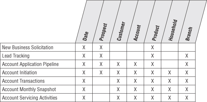
After conducting interviews with managers and analysts around the bank, the following set of requirements were developed:

• Business users want to see five years of historical monthly snapshot data on every account.
• Every account has a primary balance. The business wants to group different types of accounts in the same analyses and compare primary balances.
• Every type of account (known as products within the bank) has a set of custom dimension attributes and numeric facts that tend to be quite different from product to product.
• Every account is deemed to belong to a single household. There is a surprising amount of volatility in the account/household relationships due to changes in marital status and other life stage factors.
• In addition to the household identification, users are interested in demographic information both as it pertains to individual customers and households. In addition, the bank captures and stores behavior scores relating to the activity or characteristics of each account and household.

Dimension Triage to Avoid Too Few Dimensions

Based on the previous business requirements, the grain and dimensionality of the initial model begin to emerge. You can start with a fact table that records the primary balances of every account at the end of each month. Clearly, the grain of the fact table is one row for each account each month. Based on that grain declaration, you can initially envision a design with only two dimensions: month and account. These two foreign keys form the fact table primary key, as shown in Figure 10.2. A data-centric designer might argue that all the other description information, such as household, branch, and product characteristics should be embedded as descriptive attributes of the account dimension because each account has only one household, branch, and product associated with it.

Figure 10.2 Balance snapshot with too few dimensions.

Although this schema accurately represents the many-to-one and many-to-many relationships in the snapshot data, it does not adequately reflect the natural business dimensions. Rather than collapsing everything into the huge account dimension table, additional analytic dimensions such as product and branch mirror the instinctive way users think about their business. These supplemental dimensions provide much smaller points of entry to the fact table. Thus, they address both the performance and usability objectives of a dimensional model. Finally, given a big bank may have millions of accounts, you should worry about type 2 slowly changing dimension effects potentially causing this huge dimension to mushroom into something unmanageable. The product and branch attributes are convenient groups of attributes to remove from the account dimension to cut down on the row growth caused by type 2 change tracking. In the section “Mini-Dimensions Revisited,” the changing demographics and behavioral attributes will be squeezed out of the account dimension for the same reasons.

The product and branch dimensions are two separate dimensions as there is a many-to-many relationship between products and branches. They both change slowly, but on different rhythms. Most important, business users think of them as distinct dimensions of the banking business.

In general, most dimensional models end up with between five and 20 dimensions. If you are at or below the low end of this range, you should be suspicious that dimensions may have been inadvertently left out of the design. In this case, carefully consider whether any of the following kinds of dimensions are appropriate supplements to your initial dimensional model:

• Causal dimensions, such as promotion, contract, deal, store condition, or even weather. These dimensions, as discussed in Chapter 3: Retail Sales, provide additional insight into the cause of an event.
• Multiple date dimensions, especially when the fact table is an accumulating snapshot. Refer to Chapter 4: Inventory for sample fact tables with multiple date stamps.
• Degenerate dimensions that identify operational transaction control numbers, such as an order, an invoice, a bill of lading, or a ticket, as initially illustrated in Chapter 3.
• Role-playing dimensions, such as when a single transaction has several business entities associated with it, each represented by a separate dimension. In Chapter 6: Order Management, we described role playing to handle multiple dates.
• Status dimensions that identify the current status of a transaction or monthly snapshot within some larger context, such as an account status.
• An audit dimension, as discussed in Chapter 6, to track data lineage and quality.
• Junk dimensions of correlated indicators and flags, as described in Chapter 6.

These dimensions can typically be added gracefully to a design, even after the DW/BI system has gone into production because they do not change the grain of the fact table. The addition of these dimensions usually does not alter the existing dimension keys or measured facts in the fact table. All existing applications should continue to run without change.

Based on further study of the bank's requirements, you can ultimately choose the following dimensions for the initial schema: month end date, branch, account, primary customer, product, account status, and household. As illustrated in Figure 10.3, at the intersection of these seven dimensions, you take a monthly snapshot and record the primary balance and any other metrics that make sense across all products, such as transaction count, interest paid, and fees charged. Remember account balances are just like inventory balances in that they are not additive across any measure of time. Instead, you must average the account balances by dividing the balance sum by the number of time periods.

Figure 10.3 Supertype snapshot fact table for all accounts.

The product dimension consists of a simple hierarchy that describes all the bank's products, including the name of the product, type, and category. The need to construct a generic product categorization in the bank is the same need that causes grocery stores to construct a generic merchandise hierarchy. The main difference between the bank and grocery store examples is that the bank also develops a large number of subtype product attributes for each product type. We'll defer discussion regarding the handling of these subtype attributes until the “Supertype and Subtype Schemas for Heterogeneous Products” section at the end of the chapter.

The branch dimension is similar to the facility dimensions we discussed earlier in this book, such as the retail store or distribution center warehouse.

The account status dimension is a useful dimension to record the condition of the account at the end of each month. The status records whether the account is active or inactive, or whether a status change occurred during the month, such as a new account opening or account closure. Rather than whipsawing the large account dimension, or merely embedding a cryptic status code or abbreviation directly in the fact table, we treat status as a full-fledged dimension with descriptive status decodes, groupings, and status reason descriptions, as appropriate. In many ways, you could consider the account status dimension to be another example of a mini-dimension, as we introduced in Chapter 5: Procurement.

Household Dimension

Rather than focusing solely on the bank's accounts, business users also want the ability to analyze the bank's relationship with an entire economic unit, referred to as a household. They are interested in understanding the overall profile of a household, the magnitude of the existing relationship with the household, and what additional products should be sold to the household. They also want to capture key demographics regarding the household, such as household income, whether they own or rent their home, whether they are retirees, and whether they have children. These demographic attributes change over time; as you might suspect, the users want to track the changes. If the bank focuses on accounts for commercial entities, rather than consumers, similar requirements to identify and link corporate “households” are common.

From the bank's perspective, a household may be comprised of several accounts and individual account holders. For example, consider John and Mary Smith as a single household. John has a checking account, whereas Mary has a savings account. In addition, they have a joint checking account, credit card, and mortgage with the bank. All five of these accounts are considered to be a part of the same Smith household, despite the fact that minor inconsistencies may exist in the operational name and address information.

The process of relating individual accounts to households (or the commercial business equivalent) is not to be taken lightly. Householding requires the development of business rules and algorithms to assign accounts to households. There are specialized products and services to do the matching necessary to determine household assignments. It is very common for a large financial services organization to invest significant resources in specialized capabilities to support its householding needs.

The decision to treat account and household as separate dimensions is somewhat a matter of the designer's prerogative. Even though they are intuitively correlated, you decide to treat them separately because of the size of the account dimension and the volatility of the account constituents within a household dimension, as mentioned earlier. In a large bank, the account dimension is huge, with easily over 10 million rows that group into several million households. The household dimension provides a somewhat smaller point of entry into the fact table, without traversing a 10 million-row account dimension table. Also, given the changing nature of the relationship between accounts and households, you elect to use the fact table to capture the relationship, rather than merely including the household attributes on each account dimension row. In this way, you avoid using the type 2 slowly changing dimension technique with a 10-million row account dimension.

Multivalued Dimensions and Weighting Factors

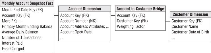
As you just saw in the John and Mary Smith example, an account can have one, two, or more individual account holders, or customers, associated with it. Obviously, the customer cannot be included as an account attribute (beyond the designation of a primary customer/account holder); doing so violates the granularity of the dimension table because more than one individual can be associated with an account. Likewise, you cannot include a customer as an additional dimension in the fact table; doing so violates the granularity of the fact table (one row per account per month), again because more than one individual can be associated with any given account. This is another classic example of a multivalued dimension. To link an individual customer dimension to an account-grained fact table requires the use of an account-to-customer bridge table, as shown in Figure 10.5. At a minimum, the primary key of the bridge table consists of the surrogate account and customer keys. The time stamping of bridge table rows, as discussed in Chapter 7: Accounting, for time-variant relationships is also applicable in this scenario.

If an account has two account holders, then the associated bridge table has two rows. You assign a numerical weighting factor to each account holder such that the sum of all the weighting factors is exactly 1.00. The weighting factors are used to allocate any of the numeric additive facts across individual account holders. In this way you can add up all numeric facts by individual holder, and the grand total will be the correct grand total amount. This kind of report is a correctly weighted report.

The weighting factors are simply a way to allocate the numeric additive facts across the account holders. Some would suggest changing the grain of the fact table to be account snapshot by account holder. In this case you would take the weighting factors and physically multiply them against the original numeric facts. This is rarely done for three reasons. First, the size of the fact table would be multiplied by the average number of account holders. Second, some fact tables have more than one multivalued dimension. The number of rows would get out of hand in this situation, and you would start to question the physical significance of an individual row. Finally, you may want to see the unallocated numbers, and it is hard to reconstruct these if the allocations have been combined physically with the numeric facts.

If you choose not to apply the weighting factors in a given query, you can still summarize the account snapshots by individual account holder, but in this case you get what is called an impact report. A question such as, “What is the total balance of all individuals with a specific demographic profile?” would be an example of an impact report. Business users understand impact analyses may result in overcounting because the facts are associated with both account holders.

In Figure 10.4, an SQL view could be defined combining the fact table and the account-to-customer bridge table so these two tables, when combined, would appear to BI tools as a standard fact table with a normal customer foreign key. Two views could be defined, one using the weighting factors and one not using the weighting factors.

Figure 10.4 Account-to-customer bridge table with weighting factor.

An open-ended, many-valued attribute can be associated with a dimension row by using a bridge table to associate the many-valued attributes with the dimension.

In some financial services companies, the individual customer is identified and associated with each transaction. For example, credit card companies often issue unique card numbers to each cardholder. John and Mary Smith may have a joint credit card account, but the numbers on their respective pieces of plastic are unique. In this case, there is no need for an account-to-customer bridge table because the atomic transaction facts are at the discrete customer grain; account and customer would both be foreign keys in this fact table. However, the bridge table would be required to analyze metrics that are naturally captured at the account level, such as the credit card billing data.

Mini-Dimensions Revisited

Similar to the discussion of the customer dimension in Chapter 8: Customer Relationship Management, there are a wide variety of attributes describing the bank's accounts, customers, and households, including monthly credit bureau attributes, external demographic data, and calculated scores to identify their behavior, retention, profitability, and delinquency characteristics. Financial services organizations are typically interested in understanding and responding to changes in these attributes over time.

As discussed earlier, it's unreasonable to rely on slowly changing dimension technique type 2 to track changes in the account dimension given the dimension row count and attribute volatility, such as the monthly update of credit bureau attributes. Instead, you can break off the browseable and changeable attributes into multiple mini-dimensions, such as credit bureau and demographics mini-dimensions, whose keys are included in the fact table, as illustrated in Figure 10.5. The type 4 mini-dimensions enable you to slice and dice the fact table, while readily tracking attribute changes over time, even though they may be updated at different frequencies. Although mini-dimensions are extremely powerful, be careful to avoid overusing the technique. Account-oriented financial services are a good environment for using mini-dimensions because the primary fact table is a very long-running periodic snapshot. Thus every month a fact table row is guaranteed to exist for every account, providing a home for all the associated foreign keys. You can always see the account together with all the mini-dimensions for any month.

Figure 10.5 Multiple mini-dimensions associated with a fact table.

As described in Chapter 4, one of the compromises associated with mini-dimensions is the need to band attribute values to maintain reasonable mini-dimension row counts. Rather than storing extremely discrete income amounts, such as $31,257.98, you store income ranges, such as $30,000 to $34,999 in the mini-dimension. Similarly, the profitability scores may range from 1 through 1200, which you band into fixed ranges such as less than or equal to 100, 101 to 150, and 151 to 200, in the mini-dimension.

Most organizations find these banded attribute values support their routine analytic requirements, however there are two situations in which banded values may be inadequate. First, data mining analysis often requires discrete values rather than fixed bands to be effective. Secondly, a limited number of power analysts may want to analyze the discrete values to determine if the bands are appropriate. In this case, you still maintain the banded value mini-dimension attributes to support consistent day-to-day analytic reporting but also store the key discrete numeric values as facts in the fact table. For example, if each account's profitability score were recalculated each month, you would assign the appropriate profitability range mini-dimension for that score each month. In addition, you would capture the discrete profitability score as a fact in the monthly account snapshot fact table. Finally, if needed, the current profitability range or score could be included in the account dimension where any changes are handled by deliberately overwriting the type 1 attribute. Each of these data elements should be uniquely labeled so that they are distinguishable. Designers must always carefully balance the incremental value of including such somewhat redundant facts and attributes versus the cost in terms of additional complexity for both the ETL processing and BI presentation.

Adding a Mini-Dimension to a Bridge Table

In the bank account example, the account-to-customer bridge table can get very large. If you have 20 million accounts and 25 million customers, the bridge table can grow to hundreds of millions of rows after a few years if both the account dimension and the customer dimension are slowly changing type 2 dimensions (where you track history by issuing new rows with new keys).

Now the experienced dimensional modeler asks, “What happens when my customer dimension turns out to be a rapidly changing monster dimension?” This could happen when rapidly changing demographics and status attributes are added to the customer dimension, forcing numerous type 2 additions to the customer dimension. Now the 25-million row customer dimension threatens to become several hundred million rows.

The standard response to a rapidly changing monster dimension is to split off the rapidly changing demographics and status attributes into a type 4 mini-dimension, often called a demographics dimension. This works great when this dimension attaches directly to the fact table along with a customer dimension because it stabilizes the large customer dimension and keeps it from growing every time a demographics or status attribute changes. But can you get this same advantage when the customer dimension is attached to a bridge table, as in the bank account example?

The solution is to add a foreign key reference in the bridge table to the demographics dimension, as shown in Figure 10.6.

Figure 10.6 Account-to-customer bridge table with an added mini-dimension.

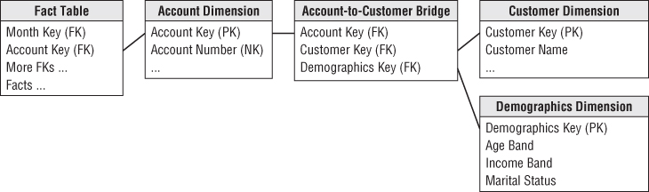
The way to visualize the bridge table is that it links every account to its associated customers and their demographics. The key for the bridge table now consists of the account key, customer key, and demographics key.

Depending on how frequently new demographics are assigned to each customer, the bridge table will perhaps grow significantly. In the above design because the grain of the root bank account fact table is month by account, the bridge table should be limited to changes recorded only at month ends. This takes some of the change tracking pressure off the bridge table.

Dynamic Value Banding of Facts

Suppose business users want the ability to perform value band reporting on a standard numeric fact, such as the account balance, but are not willing to live with the predefined bands in a dimension table. They may want to create a report based on the account balance snapshot, as shown in Figure 10.7.

Figure 10.7 Report rows with dynamic value band groups.

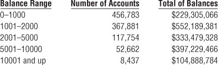
Using the schema in Figure 10.3, it is difficult to create this report directly from the fact table. SQL has no generalization of the GROUP BY clause that clumps additive values into ranges. To further complicate matters, the ranges are of unequal size and have textual names, such as “10001 and up.” Also, users typically need the flexibility to redefine the bands at query time with different boundaries or levels of precision.

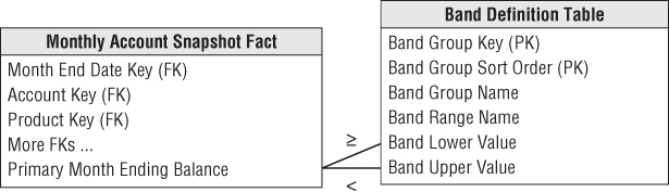
The schema design shown in Figure 10.8 enables on-the-fly value band reporting. The band definition table can contain as many sets of different reporting bands as desired. The name of a particular group of bands is stored in the band group column. The band definition table is joined to the balance fact using a pair of less-than and greater-than joins. The report uses the band range name as the row header and sorts the report on the sort order attribute.

Figure 10.8 Dynamic value band reporting.

Controlling the performance of this query can be a challenge. A value band query is by definition very lightly constrained. The example report needed to scan the balances of more than 1 million accounts. Perhaps only the month dimension was constrained to the current month. Furthermore the funny joins to the value banding table are not the basis of a nice restricting constraint because they are grouping the 1 million balances. In this situation, you may need to place an index directly on the balance fact. The performance of a query that constrains or groups on the value of a fact-like balance will be improved enormously if the DBMS can efficiently sort and compress the individual fact. This approach was pioneered by the Sybase IQ columnar database product in the early 1990s and is now becoming a standard indexing option on several of the competing columnar DBMSs.

Supertype and Subtype Schemas for Heterogeneous Products

In many financial service businesses, a dilemma arises because of the heterogeneous nature of the products or services offered by the institution. As mentioned in the introduction, a typical retail bank offers a myriad of products, from checking accounts to credit cards, to the same customers. Although every account at the bank has a primary balance and interest amount associated with it, each product type has many special attributes and measured facts that are not shared by the other products. For instance, checking accounts have minimum balances, overdraft limits, service charges, and other measures relating to online banking; time deposits such as certificates of deposit have few attribute overlaps with checking, but have maturity dates, compounding frequencies, and current interest rate.

Business users typically require two different perspectives that are difficult to present in a single fact table. The first perspective is the global view, including the ability to slice and dice all accounts simultaneously, regardless of their product type. This global view is needed to plan appropriate customer relationship management cross-sell and up-sell strategies against the aggregate customer/household base spanning all possible products. In this situation, you need the single supertype fact table (refer to Figure 10.3) that crosses all the lines of business to provide insight into the complete account portfolio. Note, however, that the supertype fact table can present only a limited number of facts that make sense for virtually every line of business. You cannot accommodate incompatible facts in the supertype fact table because there may be several hundred of these facts when all the possible account types are considered. Similarly, the supertype product dimension must be restricted to the subset of common product attributes.

The second perspective is the line-of-business view that focuses on the in-depth details of one business, such as checking. There is a long list of special facts and attributes that make sense only for the checking business. These special facts cannot be included in the supertype fact table; if you did this for each line of business in a retail bank, you would end up with hundreds of special facts, most of which would have null values in any specific row. Likewise, if you attempt to include line-of-business attributes in the account or product dimension tables, these tables would have hundreds of special attributes, almost all of which would be empty for any given row. The resulting tables would resemble Swiss cheese, littered with data holes. The solution to this dilemma for the checking department in this example is to create a subtype schema for the checking line of business that is limited to just checking accounts, as shown in Figure 10.9.

Figure 10.9 Line-of-business subtype schema for checking products.

Now both the subtype checking fact table and corresponding checking account dimension are widened to describe all the specific facts and attributes that make sense only for checking products. These subtype schemas must also contain the supertype facts and attributes to avoid joining tables from the supertype and subtype schemas for the complete set of facts and attributes. You can also build separate subtype fact and account tables for the other lines of business to support their in-depth analysis requirements. Although creating account-specific schemas sounds complex, only the DBA sees all the tables at once. From the business users' perspective, either it's a cross-product analysis that relies on the single supertype fact table and its attendant supertype account table, or the analysis focuses on a particular account type and only one of the subtype line of business schemas is utilized. In general, it makes less sense to combine data from more than one subtype schema, because by definition, the accounts' facts and attributes are disjointed (or nearly so).

The keys of the subtype account dimensions are the same keys used in the supertype account dimension, which contains all possible account keys. For example, if the bank offers a “$500 minimum balance with no per check charge” checking account, this account would be identified by the same surrogate key in both the supertype and subtype checking account dimensions. Each subtype account dimension is a shrunken conformed dimension with a subset of rows from the supertype account dimension table; each subtype account dimension contains attributes specific to a particular account type.

This supertype/subtype design technique applies to any business that offers widely varied products through multiple lines of business. If you work for a technology company that sells hardware, software, and services, you can imagine building supertype sales fact and product dimension tables to deliver the global customer perspective. The supertype tables would include all facts and dimension attributes that are common across lines of business. The supertype tables would then be supplemented with schemas that do a deep dive into subtype facts and attributes that vary by business. Again, a specific product would be assigned the same surrogate product key in both the supertype and subtype product dimensions.

If the lines of business in your retail bank are physically separated so each has its own location, the subtype fact and dimension tables will likely not reside in the same space as the supertype fact and dimension tables. In this case, the data in the supertype fact table would be duplicated exactly once to implement all the subtype tables. Remember that the subtype tables provide a disjointed partitioning of the accounts, so there is no overlap between the subtype schemas.

Supertype and Subtype Products with Common Facts

The supertype and subtype product technique just discussed is appropriate for fact tables where a single logical row contains many product-specific facts. On the other hand, the metrics captured by some business processes, such as the bank's new account solicitations, may not vary by line of business. In this case, you do not need line-of-business fact tables; one supertype fact table suffices. However, you still can have a rich set of heterogeneous products with diverse attributes. In this case, you would generate the complete portfolio of subtype account dimension tables, and use them as appropriate, depending on the nature of the application. In a cross product analysis, the supertype account dimension table would be used because it can span any group of accounts. In a single account type analysis, you could optionally use the subtype account dimension table instead of the supertype dimension if you wanted to take advantage of the subtype attributes specific to that account type.

Hot Swappable Dimensions

A brokerage house may have many clients who track the stock market. All of them access the same fact table of daily high-low-close stock prices. But each client has a confidential set of attributes describing each stock. The brokerage house can support this multi-client situation by having a separate copy of the stock dimension for each client, which is joined to the single fact table at query time. We call these hot swappable dimensions. To implement hot swappable dimensions in a relational environment, referential integrity constraints between the fact table and the various stock dimension tables probably must be turned off to allow the switches to occur on an individual query basis.

Summary

We began this chapter by discussing the situation in which a fact table has too few dimensions and provided suggestions for ferreting out additional dimensions using a triage process. Approaches for handling the often complex relationship between accounts, customers, and households were described. We also discussed the use of multiple mini-dimensions in a single fact table, which is fairly common in financial services schemas.

We illustrated a technique for clustering numeric facts into arbitrary value bands for reporting purposes through the use of a separate band table. Finally, we provided recommendations for any organization that offers heterogeneous products to the same set of customers. In this case, we create a supertype fact table that contains performance metrics that are common across all lines of business. The companion dimension table contains rows for the complete account portfolio, but the attributes are limited to those that are applicable across all accounts. Multiple subtype schemas, one of each line of business, complement the supertype schema with account-specific facts and attributes.