Chapter 6

Order Management

Order management consists of several critical business processes, including order, shipment, and invoice processing. These processes spawn metrics, such as sales volume and invoice reve*nue, that are key performance indicators for any organization that sells products or services to others. In fact, these foundation metrics are so crucial that DW/BI teams frequently tackle one of the order management processes for their initial implementation. Clearly, the topics in this case study transcend industry boundaries.

In this chapter we'll explore several different order management transactions, including the common characteristics and complications encountered when dimensionally modeling these transactions. We'll further develop the concept of an accumulating snapshot to analyze the order fulfillment pipeline from initial order to invoicing.

Chapter 6 discusses the following concepts:

• Bus matrix snippet for order management processes
• Orders transaction schema
• Fact table normalization considerations
• Role-playing dimensions
• Ship-to/bill-to customer dimension considerations
• Factors to determine if single or multiple dimensions
• Junk dimensions for miscellaneous flags and indicators versus alternative designs
• More on degenerate dimensions
• Multiple currencies and units of measure
• Handling of facts with different granularity
• Patterns to avoid with header and line item transactions
• Invoicing transaction schema with profit and loss facts
• Audit dimension
• Quantitative measures and qualitative descriptors of service level performance
• Order fulfillment pipeline as accumulating snapshot schema
• Lag calculations

Order Management Bus Matrix

The order management function is composed of a series of business processes. In its most simplistic form, you can envision a subset of the enterprise data warehouse bus matrix that resembles Figure 6.1.

Figure 6.1 Bus matrix rows for order management processes.

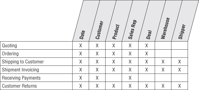
As described in earlier chapters, the bus matrix closely corresponds to the organization's value chain. In this chapter we'll focus on the order and invoice rows of the matrix. We'll also describe an accumulating snapshot fact table to evaluate performance across multiple stages of the overall order fulfillment process.

Order Transactions

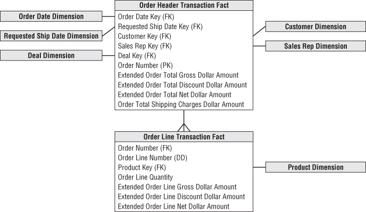
The natural granularity for an order transaction fact table is one row for each line item on an order. The dimensions associated with the orders business process are order date, requested ship date, product, customer, sales rep, and deal. The facts include the order quantity and extended order line gross, discount, and net (equal to the gross amount less discount) dollar amounts. The resulting schema would look similar to Figure 6.2.

Figure 6.2 Order transaction fact table.

Fact Normalization

Rather than storing the list of facts in Figure 6.2, some designers want to further normalize the fact table so there's a single, generic fact amount along with a dimension that identifies the type of measurement. In this scenario, the fact table granularity is one row per measurement per order line, instead of the more natural one row per order line event. The measurement type dimension would indicate whether the fact is the gross order amount, order discount amount, or some other measure. This technique may make sense when the set of facts is extremely lengthy, but sparsely populated for a given fact row, and no computations are made between facts. You could use this technique to deal with manufacturing quality test data where the facts vary widely depending on the test conducted.

However, you should generally resist the urge to normalize the fact table in this way. Facts usually are not sparsely populated within a row. In the order transaction schema, if you were to normalize the facts, you'd be multiplying the number of rows in the fact table by the number of fact types. For example, assume you started with 10 million order line fact table rows, each with six keys and four facts. If the fact rows were normalized, you'd end up with 40 million fact rows, each with seven keys and one fact. In addition, if any arithmetic function is performed between the facts (such as discount amount as a percentage of gross order amount), it is far easier if the facts are in the same row in a relational star schema because SQL makes it difficult to perform a ratio or difference between facts in different rows. In Chapter 14: Healthcare, we'll explore a situation where a measurement type dimension makes more sense. This pattern is also more appropriate if the primary platform supporting BI applications is an OLAP cube; the cube enables computations that cut the cube along any dimension, regardless if it's a date, product, customer, or measurement type.

Dimension Role Playing

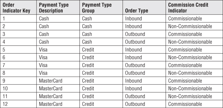
By now you know to expect a date dimension in every fact table because you're always looking at performance over time. In a transaction fact table, the primary date column is the transaction date, such as the order date. Sometimes you discover other dates associated with each transaction, such as the requested ship date for the order.

Each of the dates should be a foreign key in the fact table, as shown in Figure 6.3. However, you cannot simply join these two foreign keys to the same date dimension table. SQL would interpret this two-way simultaneous join as requiring both the dates to be identical, which isn't very likely.

Figure 6.3 Role-playing date dimensions.

Even though you cannot literally join to a single date dimension table, you can build and administer a single physical date dimension table. You then create the illusion of two independent date dimensions by using views or aliases. Be careful to uniquely label the columns in each of the views or aliases. For example, the order month attribute should be uniquely labeled to distinguish it from the requested ship month. If you don't establish unique column names, you wouldn't be able to tell the columns apart when both are dragged into a report.

As we briefly described in Chapter 3: Retail Sales, we would define the order date and requested order date views as follows:

create view order_date
  (order_date_key, order_day_of_week, order_month, …)
  as select date_key, day_of_week, month, … from date

and

create view req_ship_date
  (req_ship_date_key, req_ship_day_of_week, req_ship_month, …)
  as select date_key, day_of_week, month, … from date

Alternatively, SQL supports the concept of aliasing. Many BI tools also enable aliasing within their semantic layer. However, we caution against this approach if multiple BI tools, along with direct SQL-based access, are used within the organization.

Regardless of the implementation approach, you now have two unique logical date dimensions that can be used as if they were independent with completely unrelated constraints. This is referred to as role playing because the date dimension simultaneously serves different roles in a single fact table. You'll see additional examples of dimension role playing sprinkled throughout this book.

It's worth noting that some OLAP products do not support multiple roles of the same dimension; in this scenario, you'd need to create two separate dimensions for the two roles. In addition, some OLAP products that enable multiple roles do not enable attribute renaming for each role. In the end, OLAP environments may be littered with a plethora of separate dimensions, which are treated simply as roles in the relational star schema.

To handle the multiple dates, some designers are tempted to create a single date table with a key for each unique order date and requested ship date combination. This approach falls apart on several fronts. First, the clean and simple daily date table with approximately 365 rows per year would balloon in size if it needed to handle all the date combinations. Second, a combination date table would no longer conform to the other frequently used daily, weekly, and monthly date dimensions.

Role Playing and the Bus Matrix

The most common technique to document role playing on the bus matrix is to indicate the multiple roles within a single cell, as illustrated in Figure 6.4. We used a similar approach in Chapter 4: Inventory for documenting shrunken conformed dimensions. This method is especially appropriate for the date dimension on the bus matrix given its numerous logical roles. Alternatively, if the number of roles is limited and frequently reused across processes, you can create subcolumns within a single conformed dimension column on the matrix.

Figure 6.4 Communicating role-playing dimensions on the bus matrix.

Product Dimension Revisited

Each of the case study vignettes presented so far has included a product dimension. The product dimension is one of the most common and most important dimension tables. It describes the complete portfolio of products sold by a company. In many cases, the number of products in the portfolio turns out to be surprisingly large, at least from an outsider's perspective. For example, a prominent U.S. manufacturer of dog and cat food tracks more than 25,000 manufacturing variations of its products, including retail products everyone (or every dog and cat) is familiar with, as well as numerous specialized products sold through commercial and veterinary channels. Some durable goods manufacturers, such as window companies, sell millions of unique product configurations.

Most product dimension tables share the following characteristics:

• Numerous verbose, descriptive columns. For manufacturers, it's not unusual to maintain 100 or more descriptors about the products they sell. Dimension table attributes naturally describe the dimension row, do not vary because of the influence of another dimension, and are virtually constant over time, although some attributes do change slowly over time.
• One or more attribute hierarchies, plus non-hierarchical attributes. Products typically roll up according to multiple defined hierarchies. The many-to-one fixed depth hierarchical data should be presented in a single flattened, denormalized product dimension table. You should resist creating normalized snowflaked sub-tables; the costs of a more complicated presentation and slower intra-dimension browsing performance outweigh the minimal storage savings benefits. Product dimension tables can have thousands of entries. With so many rows, it is not too useful to request a pull-down list of the product descriptions. It is essential to have the ability to constrain on one attribute, such as flavor, and then another attribute, such as package type, before attempting to display the product descriptions. Any attributes, regardless of whether they belong to a single hierarchy, should be used freely for browsing and drilling up or down. Many product dimension attributes are standalone low-cardinality attributes, not part of explicit hierarchies.

The existence of an operational product master helps create and maintain the product dimension, but a number of transformations and administrative steps must occur to convert the operational master file into the dimension table, including the following:

• Remap the operational product code to a surrogate key. As we discussed in Chapter 3, this meaningless surrogate primary key is needed to avoid havoc caused by duplicate use of an operational product code over time. It also might be necessary to integrate product information sourced from different operational systems. Finally, as you just learned in Chapter 5: Procurement, the surrogate key is needed to track type 2 product attribute changes.
• Add descriptive attribute values to augment or replace operational codes. You shouldn't accept the excuse that the business users are familiar with the operational codes. The only reason business users are familiar with codes is that they have been forced to use them! The columns in a product dimension are the sole source of query constraints and report labels, so the contents must be legible. Cryptic abbreviations are as bad as outright numeric codes; they also should be augmented or replaced with readable text. Multiple abbreviated codes in a single column should be expanded and separated into distinct attributes.
• Quality check the attribute values to ensure no misspellings, impossible values, or multiple variations. BI applications and reports rely on the precise contents of the dimension attributes. SQL will produce another line in a report if the attribute value varies in any way based on trivial punctuation or spelling differences. You should ensure that the attribute values are completely populated because missing values easily cause misinterpretations. Incomplete or poorly administered textual dimension attributes lead to incomplete or poorly produced reports.
• Document the attribute definitions, interpretations, and origins in the metadata. Remember that the metadata is analogous to the DW/BI encyclopedia. You must be vigilant about populating and maintaining the metadata repository.

Customer Dimension

The customer dimension contains one row for each discrete location to which you ship a product. Customer dimension tables can range from moderately sized (thousands of rows) to extremely large (millions of rows) depending on the nature of the business. A typical customer dimension is shown in Figure 6.5.

Figure 6.5 Sample customer dimension.

Several independent hierarchies typically coexist in a customer dimension. The natural geographic hierarchy is clearly defined by the ship-to location. Because the ship-to location is a point in space, any number of geographic hierarchies may be defined by nesting more expansive geographic entities around the point. In the United States, the usual geographic hierarchy is city, county, and state. It is often useful to include a city-state attribute because the same city name exists in multiple states. The ZIP code identifies a secondary geographic breakdown. The first digit of the ZIP code identifies a geographic region of the United States (for example, 0 for the Northeast and 9 for certain western states), whereas the first three digits of the ZIP code identify a mailing sectional center.

Although these geographic characteristics may be captured and managed in a single master data management system, you should embed the attributes within the respective dimensions rather than relying on an abstract, generic geography/location dimension that includes one row for every point in space independent of the dimensions. We'll talk more about this in Chapter 11: Telecommunications.

Another common hierarchy is the customer's organizational hierarchy, assuming the customer is a corporate entity. For each customer ship-to address, you might have a customer bill-to and customer parent corporation. For every row in the customer dimension, both the physical geographies and organizational affiliation are well defined, even though the hierarchies roll up differently.

The alert reader may have a concern with the implied assumption that multiple ship-tos roll up to a single bill-to in a many-to-one relationship. The real world may not be quite this clean and simple. There are always a few exceptions involving ship-to addresses that are associated with more than one bill-to. Obviously, this breaks the simple hierarchical relationship assumed in Figure 6.5. If this is a rare occurrence, it would be reasonable to generalize the customer dimension so that the grain of the dimension is each unique ship-to/bill-to combination. In this scenario, if there are two sets of bill-to information associated with a given ship-to location, then there would be two rows in the dimension, one for each combination. On the other hand, if many of the ship-tos are associated with many bill-tos in a robust many-to-many relationship, then the ship-to and bill-to customers probably need to be handled as separate dimensions that are linked together by the fact table. With either approach, exactly the same information is preserved. We'll spend more time on organizational hierarchies, including the handling of variable depth recursive relationships, in Chapter 7: Accounting.

Single Versus Multiple Dimension Tables

Another potential hierarchy in the customer dimension might be the manufacturer's sales organization. Designers sometimes question whether sales organization attributes should be modeled as a separate dimension or added to the customer dimension. If sales reps are highly correlated with customers in a one-to-one or many-to-one relationship, combining the sales organization attributes with the customer attributes in a single dimension is a viable approach. The resulting dimension is only as big as the larger of the two dimensions. The relationships between sales teams and customers can be browsed efficiently in the single dimension without traversing the fact table.

However, sometimes the relationship between sales organization and customer is more complicated. The following factors must be taken into consideration:

• Is the one-to-one or many-to-one relationship actually a many-to-many? As we discussed earlier, if the many-to-many relationship is an exceptional condition, then you may still be tempted to combine the sales rep attributes into the customer dimension, knowing multiple surrogate keys are needed to handle these rare many-to-many occurrences. However, if the many-to-many relationship is the norm, you should handle the sales rep and customer as separate dimensions.
• Does the sales rep and customer relationship vary over time or under the influence of another dimension? If so, you'd likely create separate dimensions for the rep and customer.
• Is the customer dimension extremely large? If there are millions of customer rows, you'd be more likely to treat the sales rep as a separate dimension rather than forcing all sales rep analysis through a voluminous customer dimension.
• Do the sales rep and customer dimensions participate independently in other fact tables? Again, you'd likely keep the dimensions separate. Creating a single customer dimension with sales rep attributes exclusively around order data may cause users to be confused when they're analyzing other processes involving sales reps.
• Does the business think about the sales rep and customer as separate things? This factor may be tough to discern and impossible to quantify. But there's no sense forcing two critical dimensions into a single blended dimension if this runs counter to the business's perspectives.

When entities have a fixed, time-invariant, strongly correlated relationship, they should be modeled as a single dimension. In most other cases, the design likely will be simpler and more manageable when the entities are separated into two dimensions (while remembering the general guidelines concerning too many dimensions). If you've already identified 25 dimensions in your schema, you should consider combining dimensions, if possible.

When the dimensions are separate, some designers want to create a little table with just the two dimension keys to show the correlation without using the order fact table. In many scenarios, this two-dimension table is unnecessary. There is no reason to avoid the fact table to respond to this relationship inquiry. Fact tables are incredibly efficient because they contain only dimension keys and measurements, along with the occasional degenerate dimension. The fact table is created specifically to represent the correlations and many-to-many relationships between dimensions.

As we discussed in Chapter 5, you could capture the customer's currently assigned sales rep by including the relevant descriptors as type 1 attributes. Alternatively, you could use the slowly changing dimension (SCD) type 5 technique by embedding a type 1 foreign key to a sales rep dimension outrigger within the customer dimension; the current values could be presented as if they're included on the customer dimension via a view declaration.

Factless Fact Table for Customer/Rep Assignments

Before we leave the topic of sales rep assignments to customers, users sometimes want the ability to analyze the complex assignment of sales reps to customers over time, even if no order activity has occurred. In this case, you could construct a factless fact table, as illustrated in Figure 6.6, to capture the sales rep coverage. The coverage table would provide a complete map of the historical assignments of sales reps to customers, even if some of the assignments never resulted in a sale. This factless fact table contains dual date keys for the effective and expiration dates of each assignment. The expiration date on the current rep assignment row would reference a special date dimension row that identifies a future, undetermined date.

Figure 6.6 Factless fact table for sales rep assignments to customers.

You may want to compare the assignments fact table with the order transactions fact table to identify rep assignments that have not yet resulted in order activity. You would do so by leveraging SQL's capabilities to perform set operations (for example, selecting all the reps in the coverage table and subtracting all the reps in the orders table) or by writing a correlated subquery.

Deal Dimension

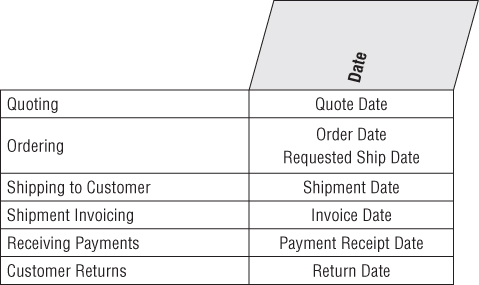
The deal dimension is similar to the promotion dimension from Chapter 3. The deal dimension describes the incentives offered to customers that theoretically affect the customers' desire to purchase products. This dimension is also sometimes referred to as the contract. As shown in Figure 6.7, the deal dimension describes the full combination of terms, allowances, and incentives that pertain to the particular order line item.

Figure 6.7 Sample deal dimension.

The same issues you faced in the retail promotion dimension also arise with this deal dimension. If the terms, allowances, and incentives are usefully correlated, it makes sense to package them into a single deal dimension. If the terms, allowances, and incentives are quite uncorrelated and you end up generating the Cartesian product of these factors in the dimension, it probably makes sense to split the deal dimension into its separate components. Again, this is not an issue of gaining or losing information because the schema contains the same information in both cases. The issues of user convenience and administrative complexity determine whether to represent these deal factors as multiple dimensions. In a very large fact table, with hundreds of millions or billions of rows, the desire to reduce the number of keys in the fact table composite key favors treating the deal attributes as a single dimension, assuming this meshes with the business users' perspectives. Certainly any deal dimension smaller than 100,000 rows would be tractable in this design.

Degenerate Dimension for Order Number

Each line item row in the order fact table includes the order number as a degenerate dimension. Unlike an operational header/line or parent/child database, the order number in a dimensional model is typically not tied to an order header table. You can triage all the interesting details from the order header into separate dimensions such as the order date and customer ship-to. The order number is still useful for several reasons. It enables you to group the separate line items on the order and answer questions such as “What is the average number of line items on an order?” The order number is occasionally used to link the data warehouse back to the operational world. It may also play a role in the fact table's primary key. Because the order number sits in the fact table without joining to a dimension table, it is a degenerate dimension.

Although there is likely no analytic purpose for the order transaction line number, it may be included in the fact table as a second degenerate dimension given its potential role in the primary key, along with the linkage to the operational system of record. In this case, the primary key for the line item grain fact table would be the order number and line number.

Sometimes data elements belong to the order itself and do not naturally fall into other dimension tables. In this situation, the order number is no longer a degenerate dimension but is a standard dimension with its own surrogate key and attributes. However, designers with a strong operational background should resist the urge to simply dump the traditional order header information into an order dimension. In almost all cases, the header information belongs in other analytic dimensions that can be associated with the line item grain fact table rather than merely being cast off into a dimension that closely resembles the operational order header record.

Junk Dimensions

When modeling complex transactional source data, you often encounter a number of miscellaneous indicators and flags that are populated with a small range of discrete values. You have several rather unappealing options for handling these low cardinality flags and indicators, including:

• Ignore the flags and indicators. You can ask the obligatory question about eliminating these miscellaneous flags because they seem rather insignificant, but this notion is often vetoed quickly because someone occasionally needs them. If the indicators are incomprehensible or inconsistently populated, perhaps they should be left out.
• Leave the flags and indicators unchanged on the fact row. You don't want to store illegible cryptic indicators in the fact table. Likewise, you don't want to store bulky descriptors on the fact row, which would cause the table to swell alarmingly. It would be a shame to leave a handful of textual indicators on the row.
• Make each flag and indicator into its own dimension. Adding separate foreign keys to the fact table is acceptable if the resulting number of foreign keys is still reasonable (no more than 20 or so). However, if the list of foreign keys is already lengthy, you should avoid adding more clutter to the fact table.
• Store the flags and indicators in an order header dimension. Rather than treating the order number as a degenerate dimension, you could make it a regular dimension with the low cardinality flags and indicators as attributes. Although this approach accurately represents the data relationships, it is ill-advised, as described below.

An appropriate alternative approach for tackling these flags and indicators is to study them carefully and then pack them into one or more junk dimensions. A junk dimension is akin to the junk drawer in your kitchen. The kitchen junk drawer is a dumping ground for miscellaneous household items, such as rubber bands, paper clips, batteries, and tape. Although it may be easier to locate the rubber bands if a separate kitchen drawer is dedicated to them, you don't have adequate storage capacity to do so. Besides, you don't have enough stray rubber bands, nor do you need them frequently, to warrant the allocation of a single-purpose storage space. The junk drawer provides you with satisfactory access while still retaining storage space for the more critical and frequently accessed dishes and silverware. In the dimensional modeling world, the junk dimension nomenclature is reserved for DW/BI professionals. We typically refer to the junk dimension as a transaction indicator or transaction profile dimension when talking with the business users.

If a single junk dimension has 10 two-value indicators, such as cash versus credit payment type, there would be a maximum of 1,024(2¹⁰) rows. It probably isn't interesting to browse among these flags within the dimension because every flag may occur with every other flag. However, the junk dimension is a useful holding place for constraining or reporting on these flags. The fact table would have a single, small surrogate key for the junk dimension.

On the other hand, if you have highly uncorrelated attributes that take on more numerous values, it may not make sense to lump them together into a single junk dimension. Unfortunately, the decision is not entirely formulaic. If you have five indicators that each take on only three values, a single junk dimension is the best route for these attributes because the dimension has only 243(3⁵) possible rows. However, if the five uncorrelated indicators each have 100 possible values, we'd suggest creating separate dimensions because there are now 100 million (100⁵) possible combinations.

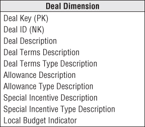
Figure 6.8 illustrates sample rows from an order indicator dimension. A subtle issue regarding junk dimensions is whether you should create rows for the full Cartesian product of all the combinations beforehand or create junk dimension rows for the combinations as you encounter them in the data. The answer depends on how many possible combinations you expect and what the maximum number could be. Generally, when the number of theoretical combinations is high and you don't expect to encounter them all, you build a junk dimension row at extract time whenever you encounter a new combination of flags or indicators.

Figure 6.8 Sample rows of order indicator junk dimension.

Now that junk dimensions have been explained, contrast them to the handling of the flags and indicators as attributes in an order header dimension. If you want to analyze order facts where the order type is Inbound (refer to Figure 6.8's junk dimension rows), the fact table would be constrained to order indicator key equals 1, 2, 5, 6, 9, 10, and probably a few others. On the other hand, if these attributes were stored in an order header dimension, the constraint on the fact table would be an enormous list of all order numbers with an inbound order type.

Header/Line Pattern to Avoid

There are two common design mistakes to avoid when you model header/line data dimensionally. Unfortunately, both of these patterns still accurately represent the data relationships, so they don't stick out like a sore thumb. Perhaps equally unfortunate is that both patterns often feel more comfortable to data modelers and ETL team members with significant transaction processing experience than the patterns we advocate. We'll discuss the first common mistake here; the other is covered in the section “Another Header/Line Pattern to Avoid.”

Figure 6.9 illustrates a header/line modeling pattern we frequently observe when conducting design reviews. In this example, the operational order header is virtually replicated in the dimensional model as a dimension. The header dimension contains all the data from its operational equivalent. The natural key for this dimension is the order number. The grain of the fact table is one row per order line item, but there's not much dimensionality associated with it because most descriptive context is embedded in the order header dimension.

Figure 6.9 Pattern to avoid: treating transaction header as a dimension.

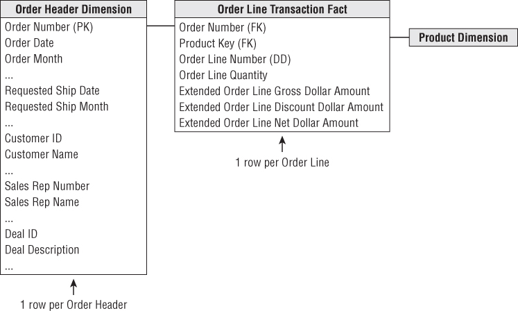
Although this design accurately represents the header/line relationship, there are obvious flaws. The order header dimension is likely very large, especially relative to the fact table itself. If there are typically five line items per order, the dimension is 20 percent as large as the fact table; there should be orders of magnitude differences between the size of a fact table and its associated dimensions. Also, dimension tables don't normally grow at nearly the same rate as the fact table. With this design, you would add one row to the dimension table and an average of five rows to the fact table for every new order. Any analysis of the order's interesting characteristics, such as the customer, sales rep, or deal involved, would need to traverse this large dimension table.

Multiple Currencies

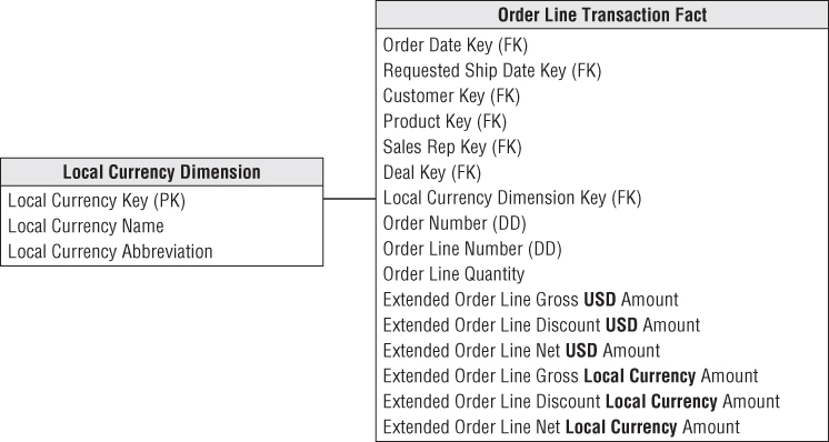
Suppose you track the orders of a large multinational U.S.-based company with sales offices around the world. You may be capturing order transactions in more than 15 different currencies. You certainly wouldn't want to include columns in the fact table for each currency.

The most common analytic requirement is that order transactions be expressed in both the local transaction currency and the standardized corporate currency, such as U.S. dollars in this example. To satisfy this need, each order fact would be replaced with a pair of facts, one for the applicable local currency and another for the equivalent standard corporate currency, as illustrated in Figure 6.10. The conversion rate used to construct each fact row with the dual metrics would depend on the business's requirements. It might be the rate at the moment the order was captured, an end of day rate, or some other rate based on defined business rules. This technique would preserve the transactional metrics, plus allow all transactions to easily roll up to the corporate currency without complicated reporting application coding. The metrics in standard currency would be fully additive. The local currency metrics would be additive only for a single specified currency; otherwise, you'd be trying to sum Japanese yen, Thai bhat, and British pounds. You'd also supplement the fact table with a currency dimension to identify the currency type associated with the local currency facts; a currency dimension is needed even if the location of the transaction is otherwise known because the location does not necessarily guarantee which currency was used.

Figure 6.10 Metrics in multiple currencies within the fact table.

This technique can be expanded to support other relatively common examples. If the business's sales offices roll up into a handful of regional centers, you could supplement the fact table with a third set of metrics representing the transactional amounts converted into the appropriate regional currency. Likewise, the fact table columns could represent currencies for the customer ship-to and customer bill-to, or the currencies as quoted and shipped.

In each of the scenarios, the fact table could physically contain a full set of metrics in one currency, along with the appropriate currency conversion rate(s) for that row. Rather than burdening the business users with appropriately multiplying or dividing by the stored rate, the intra-row extrapolation should be done in a view behind the scenes; all reporting applications would access the facts via this logical layer.

Sometimes the multi-currency support requirements are more complicated than just described. You may need to allow a manager in any country to see order volume in any currency. In this case, you can embellish the initial design with an additional currency conversion fact table, as shown in Figure 6.11. The dimensions in this fact table represent currencies, not countries, because the relationship between currencies and countries is not one-to-one. The more common needs of the local sales rep and sales management in headquarters would be met simply by querying the orders fact table, but those with less predictable requirements would use the currency conversion table in a specially crafted query. Navigating the currency conversion table is obviously more complicated than using the converted metrics on the orders fact table.

Figure 6.11 Tracking multiple currencies with daily currency exchange fact table.

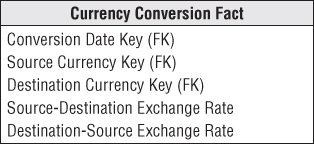
Within each currency conversion fact table row, the amount expressed in local currency is absolutely accurate because the sale occurred in that currency on that day. The equivalent U.S. dollar value would be based on a conversion rate to U.S. dollars for that day. The conversion rate table contains the combinations of relevant currency exchange rates going in both directions because the symmetric rates between two currencies are not equal. It is unlikely this conversion fact table needs to include the full Cartesian product of all possible currency combinations. Although there are approximately 100 unique currencies globally, there wouldn't need to be 10,000 daily rows in this currency fact table as there's not a meaningful market for every possible pair; likewise, all theoretical combinations are probably overkill for the business users.

The use of a currency conversion table may also be required to support the business's need for multiple rates, such as an end of month or end of quarter close rate, which may not be defined until long after the transactions have been loaded into the orders fact table.

Transaction Facts at Different Granularity

It is quite common in header/line operational data to encounter facts of differing granularity. On an order, there may be a shipping charge that applies to the entire order. The designer's first response should be to try to force all the facts down to the lowest level, as illustrated in Figure 6.12. This procedure is broadly referred to as allocating. Allocating the parent order facts to the child line item level is critical if you want the ability to slice and dice and roll up all order facts by all dimensions, including product.

Figure 6.12 Allocating header facts to line items.

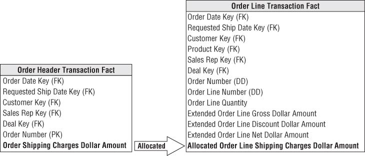
Unfortunately, allocating header-level facts down to the line item level may entail a political wrestling match. It is wonderful if the entire allocation issue is handled by the finance department, not by the DW/BI team. Getting organizational agreement on allocation rules is often a controversial and complicated process. The DW/BI team shouldn't be distracted and delayed by the inevitable organizational negotiation. Fortunately, in many companies, the need to rationally allocate costs has already been recognized. A task force, independent of the DW/BI project, already may have established activity-based costing measures. This is just another name for allocating.

If the shipping charges and other header-level facts cannot be successfully allocated, they must be presented in an aggregate table for the overall order. We clearly prefer the allocation approach, if possible, because the separate higher-level fact table has some inherent usability issues. Without allocations, you cannot explore header facts by product because the product isn't identified in a header-grain fact table. If you are successful in allocating facts down to the lowest level, the problem goes away.

Optimally, the business data stewards obtain enterprise consensus on the allocation rules. But sometimes organizations refuse to agree. For example, the finance department may want to allocate the header freight charged based on the extended gross order amount on each line; meanwhile, the logistics group wants the freight charge to be allocated based on the weight of the line's products. In this case, you would have two allocated freight charges on every order line fact table row; the uniquely calculated metrics would also be uniquely labeled. Obviously, agreeing on a single, standard allocation scheme is preferable.

Design teams sometimes attempt to devise alternative techniques for handling header/line facts at different granularity, including the following:

• Repeat the unallocated header fact on every line. This approach is fraught with peril given the risk of overstating the header amount when it's summed on every line.
• Store the unallocated amount on the transaction's first or last line. This tactic eliminates the risk of overcounting, but if the first or last lines are excluded from the query results due to a filter constraint on the product dimension, it appears there were no header facts associated with this transaction.
• Set up a special product key for the header fact. Teams who adopt this approach sometimes recycle an existing line fact column. For example, if product key = 99999, then the gross order metric is a header fact, like the freight charge. Dimensional models should be straightforward and legible. You don't want to embed complexities requiring a business user to wear a special decoder ring to navigate the dimensional model successfully.

Another Header/Line Pattern to Avoid

The second header/line pattern to avoid is illustrated in Figure 6.13. In this example, the order header is no longer treated as a monolithic dimension but as a fact table instead. The header's associated descriptive information is grouped into dimensions surrounding the order fact. The line item fact table (identical in structure and granularity as the first diagram) joins to the header fact based on the order number.

Figure 6.13 Pattern to avoid: not inheriting header dimensionality in line facts.

Again, this design accurately represents the parent/child relationship of the order header and line items, but there are still flaws. Every time the user wants to slice and dice the line facts by any of the header attributes, a large header fact table needs to be associated with an even larger line fact table.

Invoice Transactions

In a manufacturing company, invoicing typically occurs when products are shipped from your facility to the customer. Visualize shipments at the loading dock as boxes of product are placed into a truck destined for a particular customer address. The invoice associated with the shipment is created at this time. The invoice has multiple line items, each corresponding to a particular product being shipped. Various prices, discounts, and allowances are associated with each line item. The extended net amount for each line item is also available.

Although you don't show it on the invoice to the customer, a number of other interesting facts are potentially known about each product at the time of shipment. You certainly know list prices; manufacturing and distribution costs may be available as well. Thus you know a lot about the state of your business at the moment of customer invoicing.

In the invoice fact table, you can see all the company's products, customers, contracts and deals, off-invoice discounts and allowances, revenue generated by customers, variable and fixed costs associated with manufacturing and delivering products (if available), money left over after delivery of product (profit contribution), and customer satisfaction metrics such as on-time shipment.

You should choose the grain of the invoice fact table to be the individual invoice line item. A sample invoice fact table associated with manufacturer shipments is illustrated in Figure 6.14.

Figure 6.14 Shipment invoice fact table.

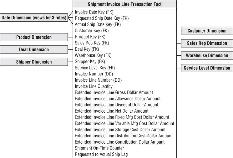
As expected, the invoice fact table contains a number of dimensions from earlier in this chapter. The conformed date dimension table again would play multiple roles in the fact table. The customer, product, and deal dimensions also would conform, so you can drill across fact tables using common attributes. If a single order number is associated with each invoice line item, it would be included as a second degenerate dimension.

The shipment invoice fact table also contains some interesting new dimensions. The warehouse dimension contains one row for each manufacturer warehouse location. This is a relatively simple dimension with name, address, contact person, and storage facility type. The attributes are somewhat reminiscent of the store dimension from Chapter 3. The shipper dimension describes the method and carrier by which the product was shipped from the manufacturer to the customer.

Service Level Performance as Facts, Dimensions, or Both

The fact table in Figure 6.14 includes several critical dates intended to capture shipment service levels. All these dates are known when the operational invoicing process occurs. Delivering the multiple event dates in the invoicing fact table with corresponding role-playing date dimensions allows business users to filter, group, and trend on any of these dates. But sometimes the business requirements are more demanding.

You could include an additional on-time counter in the fact table that's set to an additive zero or one depending on whether the line shipped on time. Likewise, you could include lag metrics representing the number of days, positive or negative, between the requested and actual ship dates. As described later in this chapter, the lag calculation may be more sophisticated than the simple difference between dates.

In addition to the quantitative service metrics, you could also include a qualitative assessment of performance by adding either a new dimension or adding more columns to the junk dimension. Either way, the attribute values might look similar to those shown in Figure 6.15.

Figure 6.15 Sample qualitative service level descriptors.

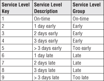
If service level performance at the invoice line is closely watched by business users, you may embrace all the patterns just described, since quantitative metrics with qualitative text provide different perspectives on the same performance.

Profit and Loss Facts

If your organization has tackled activity-based costing or implemented a robust enterprise resource planning (ERP) system, you might be in a position to identify many of the incremental revenues and costs associated with shipping finished products to the customer. It is traditional to arrange these revenues and costs in sequence from the top line, which represents the undiscounted value of the products shipped to the customer, down to the bottom line, which represents the money left over after discounts, allowances, and costs. This list of revenues and costs is referred to as a profit and loss (P&L) statement. You typically don't attempt to carry it all the way to a complete view of company profit including general and administrative costs. For this reason, the bottom line in the P&L statement is referred to as contribution.

Keeping in mind that each row in the invoice fact table represents a single line item on the invoice, the elements of the P&L statement shown in Figure 6.14 have the following interpretations:

• Quantity shipped: Number of cases of the particular line item's product. The use of multiple equivalent quantities with different units of measure is discussed in the section “Multiple Units of Measure.”
• Extended gross amount: Also known as extended list price because it is the quantity shipped multiplied by the list unit price. This and all subsequent dollar values are extended amounts or, in other words, unit rates multiplied by the quantity shipped. This insistence on additive values simplifies most access and reporting applications. It is relatively rare for a business user to ask for the unit price from a single fact table row. When the user wants an average price drawn from many rows, the extended prices are first added, and then the result is divided by the sum of the quantities.
• Extended allowance amount: Amount subtracted from the invoice line gross amount for deal-related allowances. The allowances are described in the adjoined deal dimension. The allowance amount is often called an off-invoice allowance. The actual invoice may have several allowances for a given line item; the allowances are combined together in this simplified example. If the allowances need to be tracked separately and there are potentially many simultaneous allowances on a given line item, an allowance detail fact table could augment the invoice line fact table, serving as a drill-down for details on the allowance total in the invoice line fact table.
• Extended discount amount: Amount subtracted for volume or payment term discounts. The discount descriptions are found in the deal dimension. As discussed earlier regarding the deal dimension, the decision to describe the allowances and discount types together is the designer's prerogative. It makes sense to do this if allowances and discounts are correlated and business users want to browse within the deal dimension to study the relationships between allowances and discounts.

• Extended net amount: Amount the customer is expected to pay for this line item before tax. It is equal to the gross invoice amount less the allowances and discounts.

The facts described so far likely would be displayed to the customer on the invoice document. The following cost amounts, leading to a bottom line contribution, are for internal consumption only.

• Extended fixed manufacturing cost: Amount identified by manufacturing as the pro rata fixed manufacturing cost of the invoice line's product.
• Extended variable manufacturing cost: Amount identified by manufacturing as the variable manufacturing cost of the product on the invoice line. This amount may be more or less activity-based, reflecting the actual location and time of the manufacturing run that produced the product being shipped to the customer. Conversely, this number may be a standard value set by a committee. If the manufacturing costs or any of the other storage and distribution costs are averages of averages, the detailed P&Ls may become meaningless. The DW/BI system may illuminate this problem and accelerate the adoption of activity-based costing methods.
• Extended storage cost: Cost charged to the invoice line for storage prior to being shipped to the customer.
• Extended distribution cost: Cost charged to the invoice line for transportation from the point of manufacture to the point of shipment. This cost is notorious for not being activity-based. The distribution cost possibly can include freight to the customer if the company pays the freight, or the freight cost can be presented as a separate line item in the P&L.
• Contribution amount: Extended net invoice less all the costs just discussed. This is not the true bottom line of the overall company because general and administrative expenses and other financial adjustments have not been made, but it is important nonetheless. This column sometimes has alternative labels, such as margin, depending on the company culture.

You should step back and admire the robust dimensional model you just built. You constructed a detailed P&L view of your business, showing all the activity-based elements of revenue and costs. You have a full equation of profitability. However, what makes this design so compelling is that the P&L view sits inside a rich dimensional framework of dates, customers, products, and causal factors. Do you want to see customer profitability? Just constrain and group on the customer dimension and bring the components of the P&L into the report. Do you want to see product profitability? Do you want to see deal profitability? All these analyses are equally easy and take the same analytic form in the BI applications. Somewhat tongue in cheek, we recommend you not deliver this dimensional model too early in your career because you will get promoted and won't be able to work directly on any more DW/BI systems!

Profitability Words of Warning

We must balance the last paragraph with a more sober note and pass along some cautionary words of warning. It goes without saying that most of the business users probably are very interested in granular P&L data that can be rolled up to analyze customer and product profitability. The reality is that delivering these detailed P&L statements often is easier said than done. The problems arise with the cost facts. Even with advanced ERP implementations, it is fairly common to be unable to capture the cost facts at this atomic level of granularity. You will face a complex process of mapping or allocating the original cost data down to the invoice line level. Furthermore, each type of cost may require a separate extraction from a source system. Ten cost facts may mean 10 different extract and transformation programs. Before signing up for mission impossible, be certain to perform a detailed assessment of what is available and feasible from the source systems. You certainly don't want the DW/BI team saddled with driving the organization to consensus on activity-based costing as a side project, on top of managing a number of parallel extract implementations. If time and organization patience permits, profitability is often tackled as a consolidated dimensional model after the components of revenue and cost have been sourced and delivered separately to business users in the DW/BI environment.

Audit Dimension

As mentioned, Figure 6.14's invoice line item design is one of the most powerful because it provides a detailed look at customers, products, revenues, costs, and bottom line profit in one schema. During the building of rows for this fact table, a wealth of interesting back room metadata is generated, including data quality indicators, unusual processing requirements, and environment version numbers that identify how the data was processed during the ETL. Although this metadata is frequently of interest to ETL developers and IT management, there are times when it can be interesting to the business users, too. For instance, business users might want to ask the following:

• What is my confidence in these reported numbers?
• Were there any anomalous values encountered while processing this source data?
• What version of the cost allocation logic was used when calculating the costs?
• What version of the foreign currency conversion rules was used when calculating the revenues?

These kinds of questions are often hard to answer because the metadata required is not readily available. However, if you anticipate these kinds of questions, you can include an audit dimension with any fact table to expose the metadata context that was true when the fact table rows were built. Figure 6.16 illustrates an example audit dimension.

Figure 6.16 Sample audit dimension included on invoice fact table.

The audit dimension is added to the fact table by including an audit dimension foreign key. The audit dimension itself contains the metadata conditions encountered when processing fact table rows. It is best to start with a modest audit dimension design, such as shown in Figure 6.16, both to keep the ETL processing from getting too complicated and to limit the number of possible audit dimension rows. The first three attributes (quality indicator, out of bounds indicator, and amount adjusted flag) are all sourced from a special ETL processing table called the error event table, which is discussed in Chapter 19: ETL Subsystems and Techniques. The cost allocation and foreign currency versions are environmental variables that should be available in an ETL back room status table.

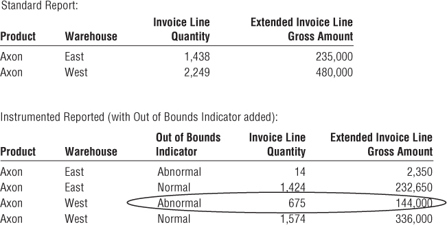
Armed with the audit dimension, some powerful queries can be performed. You might want to take this morning's invoice report and ask if any of the reported numbers were based on out-of-bounds measures. Because the audit dimension is now just an ordinary dimension, you can just add the out-of-bounds indicator to your standard report. In the resulting “instrumented” report shown in Figure 6.17, you see multiple rows showing normal and abnormal out-of-bounds results.

Figure 6.17 Audit dimension attribute included on standard report.

Accumulating Snapshot for Order Fulfillment Pipeline

The order management process can be thought of as a pipeline, especially in a build-to-order manufacturing business, as illustrated in Figure 6.18. Customers place an order that goes into the backlog until it is released to manufacturing to be built. The manufactured products are placed in finished goods inventory and then shipped to the customers and invoiced. Unique transactions are generated at each spigot of the pipeline. Thus far we've considered each of these pipeline activities as a separate transaction fact table. Doing so allows you to decorate the detailed facts generated by each process with the greatest number of detailed dimensions. It also allows you to isolate analysis to the performance of a single business process, which is often precisely what the business users want.

Figure 6.18 Order fulfillment pipeline diagram.

However, there are times when business users want to analyze the entire order fulfillment pipeline. They want to better understand product velocity, or how quickly products move through the pipeline. The accumulating snapshot fact table provides this perspective of the business, as illustrated in Figure 6.19. It enables you to see an updated status and ultimately the final disposition of each order.

Figure 6.19 Order fulfillment accumulating snapshot fact table.

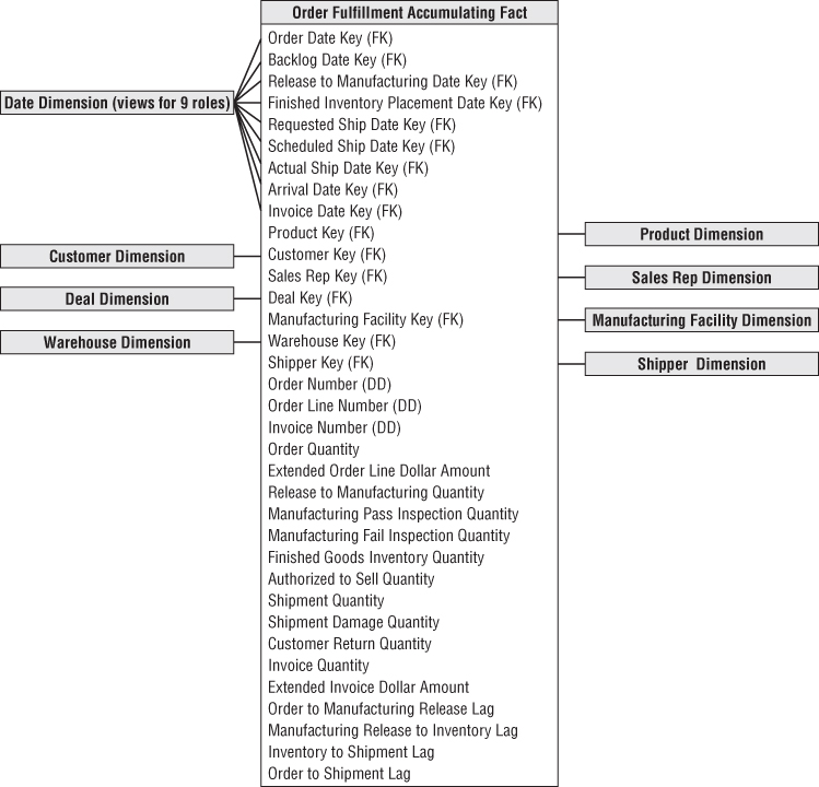
The accumulating snapshot complements alternative schemas' perspectives of the pipeline. If you're interested in understanding the amount of product flowing through the pipeline, such as the quantity ordered, produced, or shipped, transaction schemas monitor each of the pipeline's major events. Periodic snapshots would provide insight into the amount of product sitting in the pipeline, such as the backorder or finished goods inventories, or the amount of product flowing through a pipeline spigot during a predefined interval. The accumulating snapshot helps you better understand the current state of an order, as well as product movement velocities to identify pipeline bottlenecks and inefficiencies. If you only captured performance in transaction event fact tables, it would be wildly difficult to calculate the average number of days to move between milestones.

The accumulating snapshot looks different from the transaction fact tables designed thus far in this chapter. The reuse of conformed dimensions is to be expected, but the number of date and fact columns is larger. Each date represents a major milestone of the fulfillment pipeline. The dates are handled as dimension roles by creating either physically distinct tables or logically distinct views. The date dimension needs to have a row for Unknown or To Be Determined because many of these fact table dates are unknown when a pipeline row is initially loaded. Obviously, you don't need to declare all the date columns in the fact table's primary key.

The fundamental difference between accumulating snapshots and other fact tables is that you can revisit and update existing fact table rows as more information becomes available. The grain of an accumulating snapshot fact table in Figure 6.19 is one row per order line item. However, unlike the order transaction fact table illustrated in Figure 6.2 with the same granularity, accumulating snapshot fact rows are modified while the order moves through the pipeline as more information is collected from every stage of the cycle.

The accumulating snapshot technique is especially useful when the product moving through the pipeline is uniquely identified, such as an automobile with a vehicle identification number, electronics equipment with a serial number, lab specimens with an identification number, or process manufacturing batches with a lot number. The accumulating snapshot helps you understand throughput and yield. If the granularity of an accumulating snapshot is at the serial or lot number, you can see the disposition of a discrete product as it moves through the manufacturing and test pipeline. The accumulating snapshot fits most naturally with short-lived processes with a definite beginning and end. Long-lived processes, such as bank accounts, are typically better modeled with periodic snapshot fact tables.

Accumulating Snapshots and Type 2 Dimensions

Accumulating snapshots present the latest state of a workflow or pipeline. If the dimensions associated with an accumulating snapshot contain type 2 attributes, the fact table should be updated to reference the most current surrogate dimension key for active pipelines. When a single fact table pipeline row is complete, the row is typically not revisited to reflect future type 2 changes.

Lag Calculations

The lengthy list of date columns captures the spans of time over which the order is processed through the fulfillment pipeline. The numerical difference between any two of these dates is a number that can be usefully averaged over all the dimensions. These date lag calculations represent basic measures of fulfillment efficiency. You could build a view on this fact table that calculated a large number of these date differences and presented them as if they were stored in the underlying table. These view columns could include metrics such as orders to manufacturing release lag, manufacturing release to finished goods lag, and order to shipment lag, depending on the date spans monitored by the organization.

Rather than calculating a simple difference between two dates via a view, the ETL system may calculate elapsed times that incorporate more intelligence, such as workday lags that account for weekends and holidays rather than just the raw number of days between milestone dates. The lag metrics may also be calculated by the ETL system at a lower level of granularity (such as the number of hours or minutes between milestone events based on operational timestamps) for short-lived and closely monitored processes.

Multiple Units of Measure

Sometimes, different functional organizations within the business want to see the same performance metrics expressed in different units of measure. For instance, manufacturing managers may want to see the product flow in terms of pallets or shipping cases. Sales and marketing managers, on the other hand, may want to see the quantities in retail cases, scan units (sales packs), or equivalized consumer units (such as individual cans of soda).

Designers are tempted to bury the unit-of-measure conversion factors, such as ship case factor, in the product dimension. Business users are then required to appropriately multiply (or was it divide?) the order quantity by the conversion factor. Obviously, this approach places a burden on users, in addition to being susceptible to calculation errors. The situation is further complicated because the conversion factors may change over time, so users would also need to determine which factor is applicable at a specific point in time.

Rather than risk miscalculating the equivalent quantities by placing conversion factors in a dimension table, they should be stored in the fact table instead. In the orders pipeline fact table, assume you have 10 basic fundamental quantity facts, in addition to five units of measure. If you physically store all the facts expressed in the different units of measure, you end up with 50 (10 ×5) facts in each fact row. Instead, you can compromise by building an underlying physical row with 10 quantity facts and 4 unit-of-measure conversion factors. You need only four conversion factors rather than five because the base facts are already expressed in one of the units of measure. The physical design now has 14 quantity-related facts (10 + 4), as shown in Figure 6.20. With this design, you can see performance across the value chain based on different units of measure.

Figure 6.20 Physical fact table supporting multiple units of measure with conversion factors.

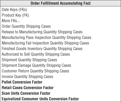
Of course, you would deliver this fact table to the business users through one or more views. The extra computation involved in multiplying quantities by conversion factors is negligible; intra-row computations are very efficient. The most comprehensive view could show all 50 facts expressed in every unit of measure, but the view could be simplified to deliver only a subset of the quantities in units of measure relevant to a user. Obviously, each unit of measures' metrics should be uniquely labeled.

Finally, another side benefit of storing these factors in the fact table is it reduces the pressure on the product dimension table to issue new product rows to reflect minor conversion factor modifications. These factors, especially if they evolve routinely over time, behave more like facts than dimension attributes.

Beyond the Rearview Mirror

Much of what we've discussed in this chapter focuses on effective ways to analyze historical product movement performance. People sometimes refer to these as rearview mirror metrics because they enable you to look backward and see where you've been. As the brokerage industry reminds people, past performance is no guarantee of future results. Many organizations want to supplement these historical performance metrics with facts from other processes to help project what lies ahead. For example, rather than focusing on the pipeline at the time an order is received, organizations are analyzing the key drivers impacting the creation of an order. In a sales organization, drivers such as prospecting or quoting activity can be extrapolated to provide visibility to the expected order activity volume. Many organizations do a better job collecting the rearview mirror information than they do the early indicators. As these front window leading indicators are captured, they can be added gracefully to the DW/BI environment. They're just more rows on the enterprise data warehouse bus matrix sharing common dimensions.

Summary

This chapter covered a lengthy laundry list of topics in the context of the order management process. Multiples were discussed on several fronts: multiple references to the same dimension in a fact table (role-playing dimensions), multiple equivalent units of measure, and multiple currencies. We explored several of the common challenges encountered when modeling header/line transaction data, including facts at different levels of granularity and junk dimensions, plus design patterns to avoid. We also explored the rich set of facts associated with invoice transactions. Finally, the order fulfillment pipeline illustrated the power of accumulating snapshot fact tables where you can see the updated status of a specific product or order as it moves through a finite pipeline.