
Chapter 8
Wideband Antennas 1
Wideband is a relative term used to describe a wide range of frequencies in a spectrum, typically from 10% to one octave and sometimes more than a decade bandwidth. This bandwidth is related to a characteristic of the antenna; in general this refers to matching, but it can also equally refer to polarization or radiation pattern.
There are essentially two main applications for wideband antennas. The first is related to the world of radar. In order to detect an object which would be hidden at certain frequencies, it is important to illuminate the targets with a wideband signal. Similarly, for reasons of accuracy in localization with pulse radars, as narrow a pulse as possible must be produced in order to increase the range resolution. It is therefore necessary in this case to widen the frequency bandwith.
The second reason is linked to the definition of channel capacity [SHA 49]. With a workable signal-to-noise ratio, capacity is thus proportional to bandwidth. The new video signal standards, such as MPEG-4, require high transmission rates and therefore a wide frequency band. Spread spectrum modulation techniques similarly require wide frequency bands. In recent years, applications classified under the acronym UWB (ultra-wideband) have become known as a result of numerous developments in localization and communication for the two reasons stated above.
There are several possible strategies for antenna design. The choice of design approach depends on the application, particularly the available space for the antenna and then by implication the frequency band and the desired gain.
The principles of antenna design will be detailed for the following:
– wideband antennas that couple the intrinsic resonances of the radiating element;
– traveling wave antennas;
– frequency independent antennas;
– UWB antennas.
8.1. Multiresonant antennas
8.1.1. Principle
In previous chapters, we have shown that microstrip antennas could be modeled using the cavity method. As the name indicates, this refers to a model using resonances of a cavity-type antenna, which is therefore intrinsically of low bandwidth. However, it is possible to attenuate this resonance with the coupling of one or more neighboring resonances in order to form a wideband antenna.
8.1.2. Widening bandwidth through resonance coupling
Figure 8.1 shows two methods which enable the bandwidth of a patch antenna fed via a coaxial connector to be widened. A slightly differently sized passive antenna (or even two for reasons of symmetry), set to a close frequency, is placed in proximity of the antenna. The proximity of this new resonance enables the bandwidth of the original antenna to be widened. This operation can be carried out either in the same plane as the antenna (a) or in superposition (b).
Figure 8.1. Different mechanisms for widening bandwidth using resonance coupling
The bandwidth obtained is thus much greater [WOO 80, SAB 83] than that observed for a microstrip structure, that can be considered as a cavity which intrinsically restricts the bandwidth of the antenna. Another method for widening bandwidth involves moving this ground plane far from the radiating part, which then becomes a reflector for the antenna.
Figure 8.2. Description of an F-probe triangular antenna
In Figure 8.2, the ground plane has been moved far from the antenna. The inductive effect created as a result of the length of the connector must therefore be balanced out. This balancing is possible using a U slot [HUY 95] or by modifying the shape of the connector. The latter solution [LEP 05, LEP 08] is shown here. The F-probe is made up of a coaxial connector and two metallic strips which are welded to its inner conductor. This passes through the ground plane. The triangular radiating element is placed over the F-probe and is fed by electromagnetic coupling.
If we calculate the input impedance of the F-probe alone and compare it to the input impedance of its two constituent L-probes, we obtain the curves represented in Figures 8.3.
We note that the F-probe strongly indicates two distinct resonances resulting from the separately considered L-probes: (H1, L1) and (H2, L2). We must also bear in mind that the coupling between the two parts of the F-probe tends to raise the values of the real and imaginary parts of the input impedance and then, as a result, make matching difficult.
Figure 8.3. Real and imaginary parts of the input impedance of F- and L-probes
Figure 8.4. Real and imaginary parts of the input impedance of F- probe with and without triangle
If we now place the metallic triangular plate over the F-probe (Figure 8.4), we see the resonance of the triangle appears, which enables the real part of the input impedance to be increased between 3 and 4 GHz, and leads to an antenna matched to 50 ohms between 3 and 5.8 GHz.
The direction of the probe and the geometry of the triangle enable a radiation similar to that of a printed wideband antenna.
8.2. Traveling wave antennas
We have just seen that widening the bandwidth of a multiresonant antenna is tricky. These resonances are linked to standing waves trapped in the antenna. If we now consider that the antenna forms a transition between a guided structure and free space, we can construct a traveling wave antenna which does not therefore produce standing waves.
The best known structure is the horn antenna. When the transition between the waveguide and free space is progressive and over a greater distance than the wavelength, there is no obstacle to propagation and the antenna is then very well matched.
8.2.1. Tapered slot antennas
Waveguides, but more so transmission lines, support wideband propagation. A transmission line is therefore the ideal support for designing a wideband antenna.
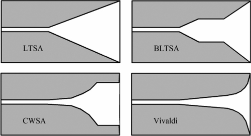
Slot antennas with progressive transitions (TSA, tapered slot antenna) provide a good example of this principle [LEW 74, GIB 79], which involves progressively widening the slot (dual slots in the case of a microstrip line) in order to be matched to the free space impedance. This transition must be as smooth as possible in order to maintain good impedance matching and leads to an aperture near to the wavelength and therefore to a directional antenna. On the basis of the geometry of their slots (see Figure 8.5), we distinguish antennas whose slots are linear (LTSA, linear tapered slot antenna), broken linearly (BLTSA, broken linear tapered slot antenna), exponential then constant (CWSA, continuous width slot antenna), or exponential (Vivaldi).
TSA antennas are matched over very wide bandwidths, from 125% to more than 170% [GUI 98]. Radiation from these is unidirectional in the substrate plane and presents a low cross-polarization level. Their directivity increases with frequency and the gains obtained by these antennas are in the range between 7 and 10 dB, depending on the type of TSA. These qualities, linked to a low dispersion in time domain, make them ideal candidates for subsurface radar applications, electromagnetic compatibility, or in metrology, since they can be arranged in an array with small gaps between antennas. They can also be used as a primary source for wideband reflectors.
Figure 8.5. Variants of tapered slot antennas
8.3. Frequency independent antennas
8.3.1. Introduction
This category of antenna covers those whose characteristics (radiation pattern, input impedance, and polarization) remain unchanged over theoretically infinite bandwidths. We saw in previous chapters how the “useful” behavior of an antenna was obtained for antenna dimensions close to the wavelength (more precisely, a half or a quarter of the wavelength). In other words, if we reduce the dimensions of an antenna by a factor of α, just its working frequency will be increased by α, but the rest of its characteristics will remain unchanged. In 1957, Rumsey [RUM 57] published a general theory on frequency independent antennas, which was based on results obtained using equiangular antennas. He showed that an antenna formed of elements, which can be deduced from each other using homothety, and uniquely defined by its angles, is frequency independent.
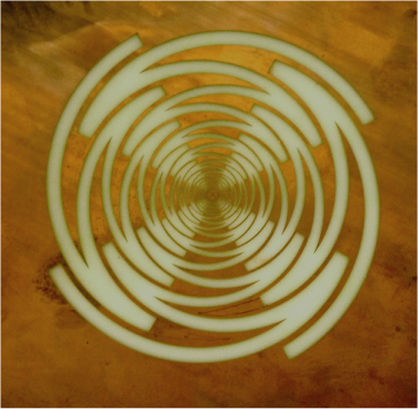
8.3.2. Equiangular antennas
The mathematical equation which satisfies the two preceding conditions is a logarithmic spiral.
Let ρ(θ) = ρ0 exp(α θ) where ρ0 is the radius centered at (θ0 = 0), and α is the coefficient regulating the expansion of the spiral (Figure 8.6).
If a section ρ0 radiates at λ0 then, for λ0>λ0 there is further a rigorously homothetic part ρ1, in the ratio λ1/λ0, which will then radiate at λ1, as λ0 radiated at λ0
In order for the antenna to have a constant impedance, independent of frequency, the width of the radiating section must remain proportional to the length of the arms, and therefore increase according to the distance of the feed point of the antenna from the center of the spiral.
Figure 8.6. Construction of a logarithmic spiral
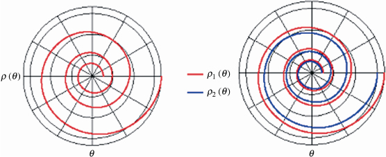
To define a plane antenna, it is therefore advisable to define the equations of two spirals which form the edges of a metallic strip: ρ1(θ) = ρ0 exp(a θ) and ρ2(θ) = ρ0 exp(α (θ − δ)) (Figure 8.7). We could equally use the same principle to construct a conical spiral [DYS 59].
The antenna is usually formed from two spirals, with the same center and with the second spiral having been obtained after a rotation of π, which result in a symmetrical structure. It is thus defined solely by its angle of rotation θ, the length of its arms, and the spiral rate 1/α (Figure 8.7).
The bandwidth of this antenna is theoretically uniquely limited by its dimensions. The central section fixes the high operating frequency, which must be low compared to the shortest wavelength (usually less than λ/8). The low operating frequency is given by the maximum length of the radiating arms. We can simply explain the principle of radiation from the antenna as follows: at the feed point, two distributions of currents in phase opposition each spread along one of the arms. The proximity of the two arms in the central area is therefore identical to a transmission line where there is no radiation. When the current propagates and moves away from the central section, radiation is produced, which reaches its maximum when these same currents are in phase. This condition is verified over a ring with a circumference equal to the wavelength. Through construction, this spiral produces a circular, or even elliptical polarized radiation when the current has not been totally radiated at the extremities of the arms (see Chapter 7). Finally, in order to excite this symmetrical antenna structure with the help of an SMA connector, a balun is very often required. Indeed, the input impedance of a logarithmic spiral antenna is typically between 75 and 100 Ω and varies depending on the thickness of the arms and the substrate used; that of a self-complementary slot spiral antenna is 188.5 Ω (60 π), in accordance with Babinet's principle. This type of wideband balun sometimes affects the performance of antennas by adding losses and limiting their bandwidth. There is however some very wideband baluns with low loss levels, for which the design has nowadays been perfected [BEG 96].
Figure 8.7. Two-arm logarithmic spiral antenna
8.3.3. Log-periodic antennas
We have seen that the relative dimensions of an equiangular spiral antenna are found to be equal for all wavelengths via a continuous transformation with properties which are preserved at all frequencies. If this transformation is periodic, rather than continuous, with a logarithmic gap between each frequency, then a log-periodic antenna is designed.
8.3.4. Sinuous antennas
Archimedean spirals (see Chapter 7) and log-spiral antennas have been used for several decades over some extremely wide bandwidths, but, in his document [DUH 87], R.H. Duhamel shows that previous attempts at utilizing more than four periodic elements in order to provide two orthogonal polarizations with radioelectrical properties and similar dimensions have been fruitless.
Figure 8.8. Dual polarized sinuous antenna

The geometry of the sinuous antenna (Figure 8.8) can be presented as a hybrid of spiral and log-periodic antennas. The geometry of the arms resembles the log-periodic antenna and allows dual polarization. When the sinuous antenna is self-complementary, its input impedance is frequency independent, as we have seen previously.
Usually this planar antenna is positioned over a cavity containing the feeding system and an absorbent whose principal function is to remove back radiation The antenna is printed onto a substrate of low permittivity The sinuous antenna is made of p cells with each cell being defined by the two parameters αp and τp (Figure 8.9)
Equation for the average fiber (Figure 8.9) of the pth cell for |ϕ| ≤ αp:
[8.1] 
Figure 8.9. Construction of the geometry of the sinuous antenna
Equation of the average fiber of the pth cell for αp ≤ |ϕ|≤ αp + δ:
[8.2] ![]()
[JOH 93] presented an approximate formula in order to calculate the lowest operating frequency of such an antenna:
[8.3] ![]()
where the angles are expressed in radians. This lowest frequency is thus limited by the exterior radius of the antenna R1 , where λL = 4 R1(α1 + δ).
As for high frequency, this is limited by the dimensions of the feeding zone. For good performance, the smallest segment of the feeding zone must be less than λH /4 in order to provide a good transition between the feeding zone and the radiating zone of the antenna.
The highest operating frequency can then be calculated from:
[8.4] ![]()
The bandwidth of the antenna can therefore be controlled by adjusting the interior and exterior diameters of the antenna. The dimensions of the feeding system limit high operating frequencies.
The radiation pattern is bidirectional (without the cavity) and symmetrical in relation to the plane of the antenna, with maximum values perpendicular to the plane and null values at the level of the plane. The half-power beamwidth varies from 60° to 100° in planes E and H. The polarization is linear and the maximum gain is typically equal to 5 dB.
Since this antenna is self-complementary, its impedance is frequency independent, while remaining raised and close to 188.5 Ω (60π), and it would be difficult to produce a very wideband feeding system enabling the transformation of characteristic impedance from 50 to 188.5 Ω.
Figure 8.10. Modified dual polarized sinuous antenna
The geometry of this sinuous antenna can be modified [BEG 00] and so it is no longer self-complementary, but even so possesses a low fluctuating input impedance, which enables matching to a far weaker characteristic impedance approaching 100 ohms (Figure 8.10). Other radiation characteristics are similar to those of the sinuous antenna.
8.4. Ultra-wideband antennas
This final category, UWB, covers a diverse range of antennas. Development of all of these antennas is linked to the publication in 2002 of a recommendation of the US Federal Communications Commission (FCC), authorizing the transmission and reception, under a certain level, of signals in a frequency band ranging from 3.1 to 10.6 GHz. This radio transmission technique consists of utilizing signals whose spectrum is spread over a wide frequency band, typically between 500 MHz and several GHz. This spectral availability enables us particularly to reach high data-rates communications and also leads to a high spatial resolution for radars.
However, the current restrictions imposed by regulatory organizations on the power transmission level limit the range of UWB communications to a few meters for high data-rates, and just a few hundred meters for low data-rates. UWB technology therefore seems naturally well placed for short-range communications (WLAN, WPAN), which offer an alternative which is at the same time low cost and low power among the existing standards.
Today, the acronym UWB brings together two standards but distinct technologies. The first has its foundations in very short pulse transmission; this is known as a monoband or Impulse Radio approach. As for the second approach, this is based on the simultaneous utilization of several carriers. This is known as the multiband technique, where the frequency band is subdivided into several subbands. The modulation used in each subband is OFDM (orthogonal frequency division multiplexing).
The pros and cons of the mono- and multiband approaches are sensitive issues and have been the subject of many debates within the regulatory organizations. One particularly significant question concerns the minimization of interference during transmission and reception in the UWB system.
The multiple band approach is particularly interesting, since carrier frequencies can conveniently be chosen in order to avoid interference with narrowband systems. It thus offers more flexibility, but requires a greater level of control in the physical layer. UWB signals in the impulse radio technique require high performance RF components (very short switching times) and very precise synchronization. UWB systems can then be developed at a relatively low cost.
Contrary to the multiband approach, which depends on techniques which are tried and trusted and readily available, impulse radio communication system architecture has given rise to numerous developments and has specifically necessitated the putting into place of new definitions and characteristics of antennas [BEG 10].
There are therefore two constraints which are strongly linked to the emergence of UWB technology: the first is the need to design compact antennas which are compatible with integration onto mobile or small-sized objects (WLAN, WPAN), and the second, for those antennas used in impulse radio mode, is not being able to change the shape of radiated pulse.
Figure 8.11. Antenna metamorphosis: from resonant to frequency independent antenna
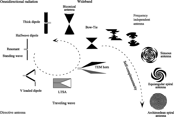
The process of antenna “metamorphosis”, shown in Figure 8.11, allows the design choice to be guided toward a Bow-Tie type of geometry, to take account of the two constraints, above.
In fact, if we examine the process which enables the transformation of a standing wave antenna into a traveling wave one, i.e. folding a dipole, loading it, transforming it in a slot line and then in a transverse electro magnetic (TEM) horn, then we observe that the size of this type of antenna becomes significant. By shortening the length of this horn and straightening the two planes, we arrive at the so-called Bow-Tie geometry.
If we now carry out a transformation of, first, a thick dipole, then a bicone one, we come back again to Bow-Tie geometry. It is interesting to observe that when the aperture angle of the Bow-Tie is 90°, this geometry is self-complementary and therefore particularly well matched to stabilizing the input impedance of a wideband antenna. We must therefore come back to Bow-Tie geometry in order to work within the two constraints which were previously set out. It goes without saying that it would be preferable to opt for a monopole structure in order to minimize the size of the antenna.
The geometries considered can be tapered, triangular, circular, elliptical, or even rectangular. This class of UWB antennas is certainly the most representative and most used in telecommunications, since they preserve the interesting characteristics of omnidirectional radiation, as well as the principles of sizing of monopole or dipole antennas, which result in relatively compact structures.
The following section is a summary of the 3rd paragraph of Chapter 5 [BEG 10].
8.4.1. Biconical and Bow-Tie antennas
The infinite biconical antenna [STU 97] can be considered to be an infinite transmission line (Figure 8.12).
Figure 8.12. Infinite biconical antenna
The input impedance of such an antenna is given by :
[8.5] ![]()
In reality, the antenna is not infinite and reflections appear at the extremities of the bicone, which limit the antenna's bandwidth. The bandwidths obtained with biconical antennas are typically from 120 to 150%. The radiation pattern is dipole-like, omnidirectional in the plane which is perpendicular to the axis of the cones and null at this axis and linearly polarized. The maximum gains are between 0 and 4 dB.
In a monopole configuration where we add a ground plane perpendicular to the axis of the half-cone, the antenna is called a discone antenna.
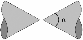
The Bow-Tie antenna is a planar version of the finite biconical antenna, which can be printed onto a substrate. This is a symmetrical structure where the currents are principally concentrated at its edges.
The Bow-Tie antenna performs less well in terms of bandwidth than the biconical antenna, being limited by the truncation of the antenna. Its input impedance varies more with frequency than that of the finite biconical antenna with the same dimensions [BAL 05]. A poorer quality of matching results from this, as well as lower bandwidth, but one which can nevertheless reach values greater than 100%.
Studies have been carried out in order to evaluate the influence of the flare angle α for a Bow-Tie antenna formed from two triangles of height H = 3 cm (Figure 8.13).
This study has been compared with the results obtained by Brown and Woodward [BRO 52] and shows the significance of this parameter on the lowest matching frequency and impedance stability of the antenna.
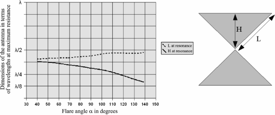
From this study, it is interesting to trace the length L in terms of the wavelength to the maximum of the real part of the impedance, as a function of the flare angle (Figure 8.14): we then observe that it is virtually equal to a half-wavelength, whatever the value of α.
In terms of radiation, the antenna presents a dipole-like radiation, i.e. omnidirectional in the plane perpendicular to that of the antenna. The resulting gains are therefore between 0 and 3 dB.
The Bow-Tie antenna can also be produced using slots in a metal plate or on a substrate [DIN 95], which enables a structure which is no longer symmetrical to be obtained. In this way, its feed can be ensured by the use of a coaxial cable without the use of a balun. However, the input impedance of such an antenna typically remains around 80 Ω.
Figure 8.13. Influence of the value of the flare angle (°) of the Bow-Tie antenna on the real part of the input impedance [BEG 10]
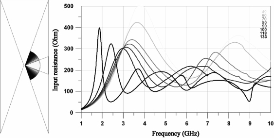
Figure 8.14. Height H and vertex L of the antenna, expressed in terms of wavelength at maximum resistance as a function of angle α [BEG 10]
8.4.2. Planar monopoles
8.4.2.1. Planar monopoles mounted over infinite ground plane
There are many works on planar monopoles mounted over infinite ground planes (or those which can be considered as infinite). Triangular and circular, and to a lesser extent square (Figure 8.15) structures are potentially antennas with wideband characteristics and their optimization leads to a wide variety of monopoles. The shape of the radiating element can also be elliptical, but too great an ellipticity ratio is detrimental to bandwidth [AGR 98].
The tilt of these elements modifies the symmetry of the unit and reduces the performances of the antenna [CHE 03]. In this section, therefore, we will solely concentrate on ground plane perpendicular planar structures.
Figure 8.15. Planar monopoles mounted over ground plane
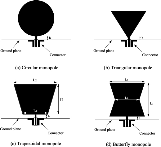
Aside from a few variations, it is easy to size up these antennas. Inherently, the low frequency is given by the height of the monopole and corresponds to a quarter wavelength. A critical parameter is the gap (h) between the monopole and the ground plane [HAM 93]. By making use of this distance, the designer can set the average input impedance of this antenna. Table 8.1 summarizes bandwidths obtained in terms of matching.
Table 8.1. Summary of performances of planar monopoles
In general, the radiation from these antennas is quasi-omnidirectional in the azimuthal plane. In the elevation plane, variations in the pattern can be significant as and when the frequency grows. A minimum of radiation appears perpendicular to the ground plane.
For all of these antennas, we must be watchful so as to preserve sufficient dimensions for the ground plane (at least greater than one wavelength at the lowest operating frequency), so as not to degrade performance of the antenna in terms of bandwidth or radiation.
However, this last condition implies that, even if the radiating part of the antenna is small, the ground plane occupies a significant space. The following section presents some examples of reduced ground plane monopole planar antennas.
8.4.2.2. Reduced ground plane planar monopoles
From the moment when the size of the ground plane is reduced, the image principle is no longer matched with the understanding of these antennas. The ground plane becomes an integral part of the antenna and can, if we pay attention to it, also radiate it.
The following figures show different strategies for reducing the size of this ground plane. There are principally two feeding methods for these antennas: using a microstrip line (Figure 8.16a), or using a coplanar waveguide (Figure 8.16b).
In reality this is not really a microstrip line or a coplanar waveguide, as these propagation supports have limited dimensions. This implies that the length of these lines will have an effect on antenna performance. It will therefore be necessary to watch that these propagation modes which are suitable for supports have had time to be established, in other words, to preserve minimum lengths for these feed lines.
Since the first solution works within this constraint, it consists of isolating the radiating part from the feeding line by using a particular T shape [FOR 04] for ground planes lateral to the coplanar waveguide (Figure 8.16c).
Decoupling between the radiating element and the feeding line limits the back current in the direction of the connector and facilitates integration with the antenna.
Figure 8.16. Strategies for optimizing the size of the ground plane
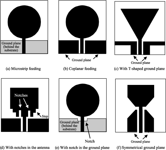
However, a minimum line length of around a quarter wavelength at the lowest frequency is nevertheless required so that the mode can be correctly established in the line. The lateral bulk of the antenna then becomes significant again and corresponds to around 2/3 of a wavelength at low frequency.
As we have underlined above, the impedance matching is dependent on the distance between the radiating part and the ground plane. One technique used to optimize matching bandwidth of the antenna is to modify the radiating part in front of the ground plane with the aid of steps or notches (Figure 8.16d) [CHO 06].
The increase in bandwidth can be spectacular, but occurs to the detriment of the radiation pattern [SU 04]. A notch in the ground plane (Figure 8.16e) also enables widening of the bandwidth [BIB 10].
Another design approach consists of designing ground planes of the same shape and size as the radiating element (Figure 8.16f) [ROB 05]. In such a case, the line no longer possesses a ground plane capable of being considered as infinite. This therefore acts uniquely as an image for the radiating element: the doublet formed as a result of this is a dipole antenna.
Thus, for this type of structure, the feed line is an integral part of the antenna and its length governs the bandwidth, which acts as a dipole.
Whether for monopole mounted over ground plane or reduced ground plane antennas, the optimization of the characteristics of radiation leads to changes in the geometry of the antenna. Today, there are a multitude of studies on the subject [PEY 05]: slot (s) insertion, trident-shaped feeding, fractal geometry, etc. However, all of these studies rely on the sizing principles that we have previously set out, and which enable any designer to initiate the design of a planar wideband antenna.
8.5. Conclusion
The design of a planar or printed antenna over a very wide frequency band is naturally more complex. The choice of geometry is guided by the application and for antennas able to transmit or receive pulses, it is advisable to consider additional parameters, such as dispersion or the fidelity factor [BEG 10].
For more classic applications, the challenge to be taken up is the necessary compromise between aperture area, gain, frequency, and bandwidth (see Chapter 9). For a compact, directive antenna, a solution favoring the resonances of the structure being studied is a good one. If the bandwidth becomes greater than the octave, it is then advisable to turn to the principles of Rumsey (defining geometry according to angles) and Babinet (self-complementary utilization) in order to guarantee performance stability as a function of frequency.
While the objective now is to design an omnidirectional and compact antenna, printed monopoles with reduced ground plane solutions are the best candidates. In terms of theoretical limits for miniaturization, let us add finally that the McLean limit remains valid for UWB, but not the Chu-Harrington limit [SCH 03].
1 Chapter written by Xavier BEGAUD.