Chapter 16

Movement of a Solid Particle in a Fluid Flow

This chapter deals with the movement of a small solid particle in a fluid flow. We start by presenting the equations governing particle movements, which we refer to as the Basset, Boussinesq, Oseen, and Tchen (BBOT) equations, to name a few key contributors to this modeling. Rather than deriving the equations, we endeavor to identify and discuss the physical meaning of the different terms: acceleration, added mass, Basset term, etc.

This approach is embodied by applying the BBOT equations to describe the behavior of a particle in three configurations of particular significance by their applications:

1. the movement of a fluid particle under the effect of gravity in a fluid at rest,

2. the movement of a particle in a unidirectional sheared fluid flow, and

3. the centrifugation of a particle in a rotating flow.

The BBOT equations allow the determination of the characteristic time with which the dynamics of a solid particle placed in a fluid flow adapts to its environment. This chapter is quite theoretical, although we have presented few derivations. This enables the reader to understand the hypotheses used in Chapters 15 (behavior of particles within gravity field) and 17 (centrifugation).

In section 16.5, we discuss the lift force applied on a particle in a unidirectional flow. This force is not taken into account by the BBOT equations. Finally, we conclude with the application of the results presented in this chapter to laminar flows, and then to turbulent flows (section 16.7).

16.1. Notations and hypotheses

We consider a spherical particle whose radius we denote by a. The mass of the particle is m_p = ρ_s4πa³ / 3, whereas m_f = ρ_f4πa³ / 3 is the mass the fluid would have had if it occupied the volume of the particle.

designates the vector describing the trajectory of the particle in the fluid. We denote by V_i(t) the three velocity components of the particle, expressed in the Cartesian coordinate system (O, x, y, z) = (O, x₁, x₂, x₃).

The particle is placed in a fluid flow which is assumed to be known. We designate by the three components of the fluid’s velocity field, which verify the Navier–Stokes equations:

[16.1]

The velocity vector is the velocity the fluid would have had at the location where the fluid particle is situated at time t, if the particle were not there. We denote by the relative velocity of the particle with respect to the fluid.

The velocity scale of the fluid flow is designated by U and its spatial scale by L. The modeling will apply to laminar as well as turbulent flows. The Reynolds number of the fluid flow,

[16.2]

(where v is the viscosity of the fluid), may be small or large.

The particle’s displacement will be calculated assuming that the particle is small. This hypothesis translates not only into the geometrical condition,

[16.3]

but also into hydrodynamic conditions specifying that the relative fluid flow with respect to the particle is a low-Reynolds-number flow. This results in three conditions on the velocity scale U of the fluid, on the scale W_p of the relative velocity of the fluid with respect to the particle, and on the angular rotational velocity ω of the particle:

[16.4]

The movement of the particle is described in the following under the four hypotheses ([16.3] and [16.4]).

16.2. The Basset, Boussinesq, Oseen, and Tchen equation

Writing the fundamental law of dynamics to describe the movement of the particle requires a balance of forces exerted on the particle. These forces are gravity on one hand and the hydrodynamic forces exerted by the fluid flow on the particle on the other hand. The particle disturbs the velocity field of the flow in its vicinity in such a manner as to verify the boundary conditions on the surface of the particle. The difficulty of the problem lies in calculating the perturbed velocity field in order to then derive therefrom the hydrodynamic forces which apply on the particle. While, as stated above, the fluid flow may be laminar or turbulent, hypotheses [16.3] and [16.4] mean that the perturbation of the velocity field caused by the particle is laminar. This is a dramatic simplification, but we will find in this chapter that the problem nevertheless remains very complex. A solution within the framework of the theory of creeping flows¹ is incomplete; the nonlinearities of the flow need to be considered in order to incorporate certain phenomena, such as the lift force exerted by a flow on a particle, into the theory. Rather than replicate here the calculations leading to the equations of motion for a small particle in a fluid flow, we merely state the final result and refer the reader to a few major publications. Our aim is first and foremost to discuss the result of this modeling, by elucidating the physical meaning of the different terms and by recalling the hypotheses of the modeling. This process will build upon the study of several application cases.

In the following we resume the notations used by Maxey and Riley (1983)² and write the Basset, Boussinesq, Oseen, and Tchen (BBOT) equations in a form that is quasi-identical to that of Maxey and Riley. This formulation is interesting insofar as it highlights the relative movement of the particle with respect to the fluid. The three components W_i (t) of the particle’s relative velocity with respect to the fluid are obtained by solving the following differential equations:

[16.5]

The differences with the equations obtained by Maxey and Riley are the corrections brought in by Auton (1987, 1988). An in-depth discussion of these equations can be found in the book by Michaelides.³

The notations appearing in [16.5] have already been introduced, with the exception of the two time derivatives. Indeed, equation [16.5] distinguishes between:

– the particle-tracking time derivative:

[16.6]

and

– the fluid-tracking time derivative:

[16.7]

both these derivatives being taken at the position of the particle center.

In the left-hand side of [16.5] are gathered the terms related to the unknowns W_i and on the right-hand side are the forcing terms associated with the velocity field of the fluid flow and with gravity. In [16.5], the numerals I–VI identify various terms that influence the movement of the particle:

Term I is the acceleration of the particle with respect to the fluid, the generic term in the equation of motion.

Term II is called the “added mass” term, as it is equivalent to adding a mass of fluid to that of the particle in order to calculate the contribution of acceleration. This only appears when the particle accelerates or decelerates with respect to the fluid, that is, in a transient regime. It is physically interpreted by the fact that, in order to accelerate the particle, some momentum also has to be imparted onto the fluid surrounding the particle. The added mass term depends heavily on the difference between the density of the particle and that of the fluid. For a particle in air, the added mass term is negligible, whereas it is significant for a particle in water. The experience of waterskiing allows us to verify that the force required to lift a stationary skier from the water is far larger than that applied if the skier starts from a pontoon. When the relative velocity of the particle with respect to the fluid becomes constant, the effect of added mass fades away, because the surrounding fluid has acquired the necessary momentum. The coefficient 1/2 associated with the added mass corresponds to the case of a spherical particle. Two terms (IIcorr terms) related to the concept of added mass also appear on the right-hand side. These corrections with respect to the formulation of Maxey and Riley are due to Auton.

Term III is the reduced weight of the particle, which is the difference between the weight of the particle and the buoyancy force that applies to it. We recall that the buoyancy force is the result of hydrostatic pressure forces applied on the particle (see Chapter 1).

Term IV is the friction force applied by the fluid on the particle in a steady-state regime. As the Reynolds number is small, we recover here the classical result associated with Stokes’ law (Chapter 15, Table 15.1). A complementary friction term (IVcorr term) appears on the right-hand side, and is linked to the shear of the velocity field of the fluid flow.

Element V consists of two terms representing pressure and inertia effects applied to the particle. These intervene in centrifugation processes, among others. It will be seen that the first term in V corresponds to the centrifugal force applied to the particle, and the second to the pressure force applied on the particle by the local pressure gradient.

Terms VI are called “Basset terms”. Indeed, they render an effect of the history of the particle’s movement with respect to the fluid. The Basset terms that appear in [16.5] are associated with an initial condition for which it is assumed that the perturbation of the velocity field is zero at time t = 0 when the particle is placed in the flow at a given location and with a given velocity, except at the particle’s surface where a non-slip condition is applied.

16.3. Movement of a particle subjected to gravity in a fluid at rest

The BBOT equations lead to the classic results on the sedimentation of a small particle within the gravity field when the surrounding fluid is at rest. They describe the acceleration of the particle which is dropped with zero velocity, and determine the characteristic time needed to reach Stokes’ fall velocity. Since u_i ≡ 0, equations [16.5] simplify into:

[16.8]

The velocity component with index 1 has been chosen to be oriented along the direction of gravity and [16.8] is the BBOT equation in that direction. In the other two directions, the equations reduce to the same equation without the right-hand side. This results in W_i (t) = 0 for i = 2 and i = 3, since W_i (t = 0) = 0. The particle’s movement occurs in the direction of gravity.

In a steady-state regime, the first two terms equal zero, thus reverting to Stokes’ law (see Table 15.1 of Chapter 15) for the fall velocity of a small spherical particle:

[16.9]

This result helps underscore the fact that the BBOT equations apply only to smallsize particles (equation [16.4]).

The transient stage during which the particle accelerates is described by the BBOT equations. Neglecting the Basset term in a first step, differential equation [16.8] simplifies into the form:

[16.10]

The solution of [16.10] is V₁(t) = W_cStokes{1−exp(−t/t_p)}, which involves the characteristic time of the transient regime:

[16.11]

Numerical applications for common cases (Table 16.1) show that the particle reaches, after a very short time, a velocity value very close to Stokes’ fall velocity. The time t_p does not depend on the nature of the force that produces the flow (in this case, gravity), since it stems from the left-hand-side terms in [16.8], but only on the properties of the fluid and the particle. It is substantially shorter for a particle in water than for a particle in air, owing to the fact that the ratio ρ_p / ρ_f is much lower in the former case. The added mass term is negligible for a particle in air. In any case, the smaller the particle, the shorter the time t_p.

The Basset term is a friction term which is added in a transient regime. In the present case, dW₁ /dτ > 0, the Basset term is positive and the friction associated with this term is added to the steady-state friction force 6πaμW₁. Because of the Basset term, the particle takes more time to reach the limiting velocity W_cStokes than evaluated as time t_p. Non-dimensionalizing the velocity by W_cStokes, and time by t_p, allows the differential equation [16.8] to be written in the following nondimensional form:

[16.12]

This formulation shows that the relative significance of the Basset term depends only on the density ratio between the particle and the fluid (more specifically, it does not depend on the size of the particle or on the viscosity of the fluid). Figure 16.1 compares the time evolution of the velocity of a particle dropped with zero velocity in the gravity field, obtained by taking into account the Basset term and by omitting it. The two cases with a Basset term correspond to a particle in air or water. It is verified that the Basset term has almost no effect for the particle in air (ρ_p / ρ_f = 3,000). For the particle in water (ρ_p / ρ_f = 3), the Basset term slows down the particle’s acceleration, but the characteristic time of the acceleration remains short (for the values indicated in Table 16.1). The characteristic time (defined by v(t′_p)/w_cStokes = (1−exp(−1))), obtained by taking into account the Basset term, is t′_p = 3.31tp.

The Basset term incorporates, via the time integral, the recent history of the particle’s movement. The quantity inside the integral allows for a damping of the history effect the further back we go in time. The Basset term becomes asymptotically zero when approaching a steady state. Indeed, if dw₁/dτ = 0 for t > t_s, we then have:

[16.13]

16.4. Movement of a particle in a steady, unidirectional shear flow

We now analyze the movement of a particle in a steady unidirectional sheared flow obtained by solving the BBOT equations. Gravity is not taken into account. The fluid flow occurs in the direction with index 1, and the velocity gradient is along the direction with index 3, which translates into:

[16.14]

denoting by z the coordinate with index 3 to facilitate interpretation of the figures.

Writing the BBOT equations does not pose any problem in this particular case. The forcing terms are zero for directions 2 and 3, which are perpendicular to the direction of the fluid flow (equations [16.16] and [16.17]). In the direction of the fluid flow (equation [16.15]), non-zero forcing terms related to the gradient of the fluid flow (IIcorr and IVcorr terms in [16.5]) remain. For element V in [16.5], the term related to the fluid-tracking material derivative is zero since u₃ ≡ 0. Only the term related to the particle-tracking material derivative is non-zero. This is written by bringing in the relative velocity component, since W₃ =V_3.

[16.15]

[16.16]

[16.17]

The solutions of equations [16.16] and [16.17] are of the same nature as those obtained in section 16.3. The relative velocities W₂ and W₃ rapidly tend toward zero if there is an initial velocity in these directions. The characteristic time of the transient regime is identical to [16.11]:

[16.18]

Thus, the particle’s movement aligns itself very rapidly with the direction of the fluid flow.

equation [16.15] is solved in a similar manner. The velocity of the particle in direction 1 becomes asymptotically, in a steady-state regime,

[16.19]

The shear of the fluid flow produces a relative velocity of the particle with respect to the fluid. The difference is often very small. For a Poiseuille flow, for example, the velocity of the particle is less than the velocity of the fluid, but the correction is of the order of (a / L)², which is very small (equation [16.3]).

It is important to analyze the forces exerted on the particle in terms of drag force and lift force. The drag force F_// is the component of the hydrodynamic force exerted on the particle, projected onto the direction of the particle’s relative velocity with respect to the fluid, while the lift force F_⊥ is the component perpendicular to that direction. In Figure 16.2 we specify the notations and sketch the balance of forces exerted on the particle by the fluid flow. When the directions of the particle and fluid velocities are not parallel, the lift and drag are not always simple to interpret from a physical point of view. On the other hand, when the movement of the particle has aligned with the direction of the fluid flow, it is important to note that the BBOT equations correspond to a lift force that becomes zero. The shear of the fluid flow produces only a drag force:

[16.20]

which is balanced by the friction resulting from the relative movement of the particle with respect to the fluid.

16.5. Lift force applied to a particle by a unidirectional flow

The example discussed in the previous section using the BBOT equations shows that the trajectory of a solid particle tends to align with the direction of the fluid flow. The fluid flow does not exert a lift force on the particle, even if it possesses a velocity gradient in the direction perpendicular to that of the flow. This result contradicts some observations of fluid mechanics. The lack of a lift force, for example, does not allow fluid particles to migrate in the direction perpendicular to the direction of the flow, or the fluid to pick up a particle lying on a wall. The study of the lift force has given rise to a considerable amount of research, of which we summarize a few important results. The reader will find in the book by Michaelides⁴ a precise history of that work. In the following, we only mention a few essential articles.

We shall study successively the lift force applied on a particle in a fluid flow in an infinite medium and then the case where the particle is near a wall.

16.5.1. Lift force exerted on a particle in a fluid flow in an infinite medium

Figure 16.3 depicts two configurations for which theoretical evaluations of the lift force are established. The case of Figure 16.3(b) has prompted numerous studies, aiming at the following:

– Understanding how the shearing of the velocity field produces a lift force. We will focus on the case where the shear is uniform ( du_x / dz = G = constant).

– Understanding the role of the particle’s rotation. Two cases are usually considered: (i) the particle can rotate freely without friction about an axis that is perpendicular to the plans of the flow; the shear of the fluid flow then causes the particle to rotate; and (ii) the particle is prevented from rotating.

– Understanding the effect of the relative movement of the particle with respect to the fluid, in the direction of the fluid flow. W₁ denotes the relative velocity of the particle with respect to the fluid.

The first case (Figure 16.3(a)) is that of the very classic Magnus effect for a high-Reynolds-number flow. If a rotation with angular velocity ω about the Oy axis is forced on a particle of radius a placed in a uniform fluid flow u₀ (such that u₀a/v >>1) along the Ox direction, a lift force is generated on the particle in the Oz direction:

[16.21]

The rotation vector is for the configuration of Figure 16.3(a). Viscosity is absent from relation [16.21], and the force is of an inertial nature. While the rotation of the particle produces, because of viscous friction, a rotating movement of the fluid around the particle, in a steady-state regime the kinematics of the flow is independent from viscosity. The pressure along the streamlines that pass the particle is calculated using Bernoulli’s theorem, and only the velocity on the surface of the particle intervenes to vary the pressure. The Magnus effect is well known to aerodynamicists, since it is the analogy with the potential flow past a rotating cylinder that explains the lift applied to a thin aircraft wing at incidence. It also explains the effects obtained when a tennis player uses topspin on a ball or slices it.⁵

Let us now consider the configuration of Figure 16.3(b). The fluid, in an infinite medium, has a constant-shear flow (du_x / dz = G). The particle has a relative movement with velocity W₁ in the Ox direction of the fluid flow. Similar hypotheses to [16.4], meaning that the particle is small, are:

[16.22]

The theoretical difficulties in calculating the lift force are significant. It was proved by Bretherton⁶ that no lift force is exerted on a body of revolution by a parallel flow if we remain within the scope of the theory of creeping flows (removing nonlinear terms from the Navier–Stokes equations). It is therefore necessary to take into account the inertial (nonlinear) terms. This difficulty had been identified in 1910 by Oseen, who had indicated that the nonlinear terms cannot be neglected if the location is sufficiently far from the center of the particle. For the characteristics of the flow under consideration, we naturally introduce the two length scales related to the slip velocity:

[16.23]

or to the shear:

[16.24]

The solution for the flow around the sphere cannot be calculated properly beyond these distances without taking into account the nonlinearities associated respectively to the relative velocity of the particle with respect to the fluid or to the shear of the fluid flow. The conditions [16.22] whereby the particle is small simply mean that L_W1 / a>>1 and L_G / a>>1.

Mathematical developments solving for the flow around the particle distinguish the inner region within the distance min{Lw₁,L_G} from the center of the particle, where the flow is essentially governed by viscosity, and the outer region beyond that distance, where nonlinearities have to be taken into account. The general solution of the problem needs to merge the solutions between both domains.

Saffman⁷ showed that viscosity produces, for the configuration of Figure 16.3(b), a lift force:

[16.25]

oriented as indicated in Figure 16.3(b) in terms of the directions of the flow and shear. The ratio of the lift force to the drag force (of magnitude 6πμW ₁a ) is of the order of ; it is therefore small compared to the drag force. The lift force obtained by Saffman is identical whether the particle can rotate freely or its rotation is blocked. If the particle can rotate freely, its rotational speed establishes itself at ω = G/2, so as to cancel out, in a steady-state regime, the rotation torque exerted by the fluid flow on the particle. The independence of the lift force from the rotation of the particle can be understood by noting that the ratio of the lift force after Saffman [16.25] to the lift force related to the Magnus effect is of the order of . Saffman’s mathematical developments are subject to the condition (i.e. LG << L_W1 ), which, in practice, is restrictive with respect to typical conditions. Either the fluid’s viscosity has to be very high or the relative velocity of the particle with respect to the fluid has to be particularly small.

McLaughlin generalized Saffman’s work for an arbitrary value of the ratio (Saffman studied the case where ε = ∞). The lift force is expressed in the form

[16.26]

In Table 16.2 we provide a few values of functional J(ε). For ε tending toward infinity, 9J(ε = ∞) / π = 6.46, so that [16.26] is very close to Saffman’s result. The factor J(ε) decreases by a factor of 100 when ε diminishes from infinity to 0.25. The lift force changes direction for ε ≈ 0.22. J(ε) tends toward zero when ε tends toward zero (the shear goes to zero). For ε > 0.25, the value of J(ε) is sufficiently large for the lift force to differ only slightly depending on whether the particle can rotate freely or its rotation is prevented. This no longer holds for ε <0.25 as the absolute value of J(ε) becomes very small.

Also, for the configuration of Figure 16.3(b), Auton⁸ obtained the lift force:

[16.27]

which is worthy of some comment, as the hydrodynamic conditions differ from those studied previously. Auton’s calculation is inviscid, with the fluid slipping on the surface of the particle. Result [16.27] differs from that of the Magnus effect, despite the similarity of the equations, because the calculation does not take into account a possible rotation being imparted to the particle. The lift force obtained by Auton results from the deformation in the velocity curl field produced by the presence of the spherical particle. The calculation is performed under the sole condition that the shear is small, that is, Ga/W₁ <<1. Auton’s result applies mainly to large-size particles and not to small particles in the sense of [16.4]. Viscosity cannot be neglected for small particles, and it is found that the lift force given by relation [16.26] or [16.27] is larger than what Auton’s calculation predicts, unless J(ε) is small in the conditions considered.

16.5.2. Lift force exerted on a particle in the vicinity of a wall

The proximity of a wall influences the lift force applied on a particle. Figure 16.4 shows three configurations studied more specifically.

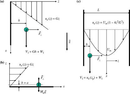
Configuration Figure 16.3(a) is modified, compared to that of Figure 16.3(b), by the addition of a plane wall at z = 0. The distance from the center of the particle to the wall is denoted by h. The diagram is rotated by 90° with respect to Figure 16.3 in order to represent conventionally the case where the direction of the flow is parallel to the direction of gravity. Thus, if the particle is denser than the fluid, this configuration depicts the simple case where the influence of the wall on the gravitational sedimentation of the particle is studied.

A comparison of the distance h between the center of the particle and the wall with the scales (equations [16.23−16.24]) helps assess the nature of the effect of the wall on the lift force applied to the particle. If h << min {L_w1, L_G}, the wall crosses the inner zone of the flow around the particle. The solution in that zone, for which the contribution of the inertial terms is negligible, can satisfy both the boundary conditions on the particle and on the wall. If h ≈ min{Lw₁, L_G}, the wall is situated in the outer zone of the flow around the particle. The effect of the wall on the lift force involves the inertial terms. Finally, if h >> max {L_w1, L_G }, then the wall is too far to alter the lift force.

When the wall is situated in the inner zone around the particle and the relative velocity W₁ is non-zero (h << min{L_w1,L_G}), Cherukat and McLaughlin⁹ have established that the lift force takes on the form:

[16.28]

with the length ratio κ = a/h (note that κ < 1 necessarily) and the velocity ratio of the fluid flow to the relative velocity of the particle Λ_G= Ga/W₁. We have Λ_G > 0 if the particle is faster than the fluid (as in Figure 16.4(a)) and Λ_G < 0 if the reverse is true. Expression [16.28] has the remarkable property of being independent of viscosity. Results of numerical calculations were used by Cherukat and McLaughlin to tabulate the functional I(κ,Λ_g ) into the following correlations:

[16.29]

for a non-rotating sphere, and:

[16.30]

when the sphere can rotate freely under the effect of shear. The figures plotted in the article by Cherukat and McLaughlin help interpret relations [16.29] and [16.30]. When the sphere is sufficiently far from the wall (h/a > 5), the wall repels the particle (I > 0) if the particle is moving faster than the fluid (Λ_G < 0), whereas it attracts it in the reverse situation. When the particle is near the wall (h/a close to 1), the wall repels the particle (I> 0) irrespective of the sign of Λ_G (and therefore of the sign of the relative velocity W₁), except inside an interval of positive values of Λ_G (between 0 and 2.5) for which slightly negative values of I are obtained. The rotation of the particle is generally found to have little impact on the lift force.

The particular case for which the relative velocity W₁ is zero is worth discussing. The term “neutral particles” is used, in the sense that, for the configuration of Figure 16.4(a), the particle has the same density as the fluid, and therefore does not settle in the gravity field. The asymptotic limit of [16.28], associated with the correlation [16.29] or [16.30], when W₁ tends toward zero, is written as:

[16.31]

for a sphere that is prevented from rotating, and:

[16.32]

for a sphere that can rotate freely. As κ = a / h < 1, it can be verified that the force is always oriented in the same direction as , which means that the shear in the velocity field produces a force which repels the particle away from the wall.

In the case where the wall is situated in the outer region with respect to the center of the particle (h > max {L_W1, L_G}), a previous study by McLaughlin¹⁰ shows that the wall exerts an additional force which attracts or repels the particle depending on whether the particle is moving parallel to the wall faster or slower than the fluid. This force:

[16.33]

is added to the lift force [16.26] calculated by McLaughlin (1991) in an infinite medium. The minus sign in [16.33] indicates that the additional force is oriented in the opposite direction to the shear-induced lift force (when J(ε) > 0). The wallinduced additional lift force decreases to zero when h increases.

Cherukat’s and McLaughlin’s relations also enable the determination of the lift force exerted by a boundary layer flow on a particle that is settled at rest on a horizontal plane (Figure 16.4(b)). In that case, κ = 1 and Λ_G = −1 since V₁ = Ga + W₁ = 0. By substituting these values, we infer from [16.29] that I = 9.29 and:

[16.34]

This expression enables the determination of the conditions for which the fluid flow entrains the particle in suspension, if the particle is denser than the fluid and the gravity force is perpendicular to the wall (Figure 16.4(b)). For that to occur, the lift force must exceed the reduced weight of the particle, which leads to the condition:

[16.35]

The gradient of the velocity field determines the takeoff condition.

There is considerable literature concerning the lift force exerted on a particle in a Poiseuille flow. The current development of microfluidics opens new prospects for such works, which have historically been strongly motivated by applications in the medical field for understanding the transport of blood cells in arteries and veins. We consider the situation of Figure 16.4(c) where the walls are parallel to the direction of gravity. The pioneering experiments of Segré and Silberberg¹¹ have demonstrated the lateral migration of rigid neutral particles (equality of densities between the fluid and particles). An inhomogeneous distribution of particles occurs in a cross section of the flow, with a maximum concentration around the radial position r = 0.6R. Work on the lift force exerted on a particle in a homogeneously sheared flow (configuration of Figure 16.4(a)), which we have previously mentioned, provides the mathematical framework to study the case of Poiseuille flows, with the concepts of inner and outer zones around the particle for discussing the phenomena producing the lift force. It is however not sufficient to completely study the case of Poiseuille flows. Shear decreases linearly in a Poiseuille flow when moving from the wall toward the center of the pipe. In a similar manner to what is demonstrated by Cherukat and McLaughlin (1994) in a homogeneously sheared flow, it is observed in a Poiseuille flow that the wall exerts a lift force which repels a particle located near the wall. In the central part of the pipe, the shear becomes small. The ratio of the inertial scale L_W1 to the inertial scale L_G becomes small at the center of the pipe. Referring to the work of McLaughlin (1991) for a homogeneously sheared flow in an infinite medium, we can understand that the lift force exerted on a particle, although smaller in magnitude in the central part of the pipe than it is near the wall, pushes toward the wall a particle situated in the central part whereas it repels it away from the wall when it is close to it. This is indeed the phenomenology observed experimentally by Segré and Silberberg and highlighted by theoretical studies. We limit ourselves to citing a few important articles,¹² from which it is easy to reconstitute a comprehensive bibliography. The calculations by Asmolov (1999) highlight the difference in the direction and order of magnitude of lift forces between the near-wall region and the central part of the pipe for different values of the Reynolds number Re_c = U_mL /ν of the Poiseuille flow (U_m is the velocity maximum of the Poiseuille flow, Figure 16.4(c)). This work builds on previous research by Schoenberg and Hinch (1989) and Hogg (1994). Schoenberg and Hinch’s work, in particular, sets out the specificity of the Poiseuille flow. The curvature of the Poiseuille flow causes a pressure gradient effect, which also contributes to repelling particles situated in the central part of the pipe toward the walls.

16.6. Centrifugation of a particle in a rotating flow

To conclude our inventory of a few application cases of the BBOT equations, we now consider a rotating flow about Oz axis, omitting gravity. In the cylindrical coordinate system (Figure 16.5), the only non-zero velocity component is the azimuthal component. We consider a velocity field for the flow in the form:

[16.36]

The rotating flow is the combination of a solid-body rotation flow and a vortex flow. As will be seen in Chapter 17, this case corresponds to many configurations for which centrifugal separation is implemented. Theoretically speaking, such flows verify the property . This property greatly simplifies the BBOT equations. It also makes it easier to identify the terms and mechanisms responsible for centrifugal separation.

As the BBOT equations [16.5] are written in the Cartesian coordinate system (O,x₁,x₂,x₃), the first step is to transcribe the velocity field into the Cartesian coordinate system:

[16.37]

In this configuration, the BBOT equations [16.5] are written as:

[16.38]

Since Δ ≡ 0, the only non-zero quantities on the right-hand side of [16.5] pertain to terms V and IIcorr. Analyzing the three terms on the right-hand side of [16.38] leads to the identification of the centrifugal separation mechanism. These terms equal zero for the direction parallel to the axis of rotation (i = 3). For i = 1 and i = 2, the first two terms are written as:

[16.39]

Bringing to the fore the relative velocities of the particle with respect to the fluid, W₁ = V₁ − u₁ and W₂ = V₂ − u₂, leads to:

[16.40]

so that the right-hand sides of equation [16.38] for i = 1 and i = 2 are:

[16.41a]

[16.41b]

Substituting the velocity field [16.37] into [16.41], we can write [16.38] in the form:

[16.42a]

[16.42b]

[16.43]

The next step is to transcribe these equations into the cylindrical coordinate system by expressing the BBOT equations for the radial and azimuthal components of the particle’s velocity:

[16.44]

Likewise, the radial and azimuthal components of the particle’s relative velocity with respect to the fluid are:

[16.45]

The BBOT equation for the radial component is obtained by multiplying respectively [16.42a] and [16.42b] by x₁ / r and x₂ / r, then summing the two equations. Lengthy but not especially difficult calculations yield the following equation, in which the relative velocities in the Cartesian coordinate system W₁ and W₂ are eliminated to bring forth the relative velocities W_r and W_θ in the cylindrical coordinate system:

[16.46]

In order to simplify the calculations, we have omitted the Basset terms, which have been found not to alter the nature of the physics. These essentially amount to an additional friction term, which slows down the adaptation of the particle’s movement to the surrounding flow, but this adaptation remains very rapid anyway. On the left-hand side, the second term appears when the acceleration is expressed while changing the reference frame. Transferring this term to the right, we infer:

[16.47]

The acceleration term in [16.47] is written on the basis of coordinates r and θ and the radial and azimuthal components of the particle’s velocity, since the coordinate change verifies with [16.44]:

[16.48]

By a similar procedure, the BBOT equation for the azimuthal component is obtained by multiplying respectively [16.42a] and [16.42b] by −x₂ /r and x₁ /r, and then summing the two equations. This leads to:

[16.49]

The equation for the axial component remains [16.43].

The left-hand-side terms in equations [16.43], [16.47], and [16.49] are in identical form to those derived when we studied the fall of a small particle within the gravity field (section 16.3) or its displacement in a unidirectional fluid flow (section 16.4). The time periods characterizing the acceleration phase of the particle are identical (equations [16.11] and [16.18]). We recall that these were short. Our discussion regarding the Basset terms (section 16.3) also transposes to the case of centrifugation.

We conclude from [16.43] that the relative velocity of the particle W₃ = W_z in the direction of the axis of rotation goes to zero rapidly if the W_z was non-zero at the initial time. As the velocity u_z of the flow in that direction is zero [16.36], the trajectory of the particle is rapidly confined to a particular plane perpendicular to the axis of rotation.

The forcing terms for the relative movement in that plane of the particle with respect to the fluid bring forth in [16.47] and [16.49] terms of different natures:

– The (m_p − m_f)u_θ² /r term in [16.47] is the one that causes the centrifugation of particles in the axial direction (equation [16.47]). The particle moves away from the axis of rotation if ρ_p > ρ_f. It moves toward it if the reverse is true. The term m_pu_θ² /r corresponds to the centrifugal force. The term − m_fu_θ² /r is the pressure force exerted by the rotating flow on the particle. We will establish that in Chapter 17 (section 17.3). The term (m_p −m_f )u_θ²/r is essentially balanced with the friction term 6πaμW_r, thus determining the relative radial velocity W_r of centrifugation.

– The other terms appearing in [16.47] and [16.49] are akin to Coriolis forces for movement in a rotating reference frame. Transposing the criteria [16.4] according to which the flow has a low Reynolds number, the rotating flow must be such that:

Under these conditions, we verify that these Coriolis terms are small compared to the centrifugation terms. The relative velocity of the particle in the azimuthal direction is also small relative to the relative velocity in the radial direction (W_θ / W_r <<1).

In a rotating flow, the BBOT equations therefore describe a centrifugation movement of a small particle, the characteristics of which are driven by rather simple mechanisms. The duration of the transient regime before equilibrium between the centrifugal forcing term and the friction is very short. The centrifugation process is described approximately by:

[16.50]

The difference between the centrifugal force and the pressure force exerted by the rotating flow on the particle, which generates centrifugation, is balanced by the (drag-like) friction force associated with the relative radial movement of the particle with respect to the fluid. This result will be used in Chapter 17.

16.7. Applications to the transport of a particle in a turbulent flow or in a laminar flow

The examples of application of the BBOT equations discussed in this chapter allow some useful guidance to be drawn in order to elucidate and justify the hypotheses formulated in the other chapters of this part. By keeping in mind that these equations are obtained for small particles, the following points should be emphasized:

– The characteristic time t_p of the transient regime leading to the adaptation of the particle’s movement in the fluid flow is short. Mechanical equilibrium is reached very rapidly between the forcing terms of the particle’s movement and the viscous drag force resisting the relative movement of the particle with respect to the fluid. We have used this result in Chapter 15 by assuming, in the context of gravitational separation, that the relative velocity of a particle with respect to the fluid is equal to the fall velocity of a particle. We shall revert to it in Chapter 17 (section 17.3) when discussing centrifugal separation.

– The Basset terms (terms VI in equation [16.5]) are additional drag terms which intervene during a transient regime. Their significance depends on the value of the density ratio ρ_p / ρ_f. They are negligible for particles in a gas. They are not negligible when the densities of the particle and fluid are comparable, although they do not modify the order of magnitude of the characteristic time t_p of the transient regime, which remains very short. For this reason, they are often ignored.

– The BBOT equations have enabled the introduction of the added mass effect, which intervenes during the acceleration and deceleration phases of the particle in the fluid. In a transient regime, the added mass is essential for a bubble in a liquid (ρ_p / ρ_f <<1), because the bubble has to transmit momentum to the liquid in order to be able to accelerate itself.

– The centrifugation of a particle in a rotating flow is governed by the centrifugal force linked to the rotation of the fluid flow and by the pressure force exerted by the fluid flow on the particle (terms V in [16.5]). We will use this result in Chapter 17 (section 17.3).

– For a steady unidirectional sheared flow, we have found (section 16.4) that the trajectory of a small fluid particle rapidly aligns with direction of the fluid flow. The hydrodynamic force exerted on the fluid particle is essentially the drag force −6πμaW_j. We have used this result on various occasions in this part (Chapter 15, section 15.4 regarding Brownian motion, among others). The BBOT equations do not bring forth a lift force. Our review of lift forces (section 16.5) shows that, for small particles, the magnitude of the lift force is small compared to that of the drag force. This explains why the lift force is not taken into account in the BBOT equations.

The application of the results presented in this chapter is differentiated depending on whether the movement of a particle is considered in a laminar or in a turbulent flow.

16.7.1. Application to laminar flows

The development of microfluidics makes the study of the movement of a small particle in a laminar flow an especially dynamic topic nowadays. The contents of this chapter, without having gone into the detail of theoretical developments, show the complexity and difficulty of the subject. A pertinent modeling of the movement of a particle, in order to encompass phenomena such as the resuspension of particles from walls or the migration of particles in a direction perpendicular to the flow streamlines, should incorporate the lift force exerted on a particle, even though it is much weaker than the drag force.

16.7.2. Application to turbulent flows

For a particle in a turbulent flow whose characteristic scales of velocity and length are denoted respectively by u_rms and ℓ_t, the results described in this chapter mean that the movement of the particle aligns with the direction of the turbulent fluid flow if the characteristic time t_p of the transient regime, during which the movement of the particle adapts to the surrounding fluid flow, is small compared to the characteristic time τ_t = l_t /u_rms of turbulence, which is often the case (t_p << τ_t). In such a situation, the BBOT equations justify modeling the transport of a particle as a random walk process, wherein the movement of the particle adapts rapidly to follow the variations of the turbulent flow. The turbulent diffusion process described in Chapter 8 results in the migration of particles perpendicularly to the direction of the mean flow much faster than the lift force contributes to it. That is the reason why we have presented in Chapter 15 (section 15.5) the sustenance in suspension of particles within a turbulent flow as a balance between the sedimentation flux and the turbulent diffusion flux. The lift force remains essential for determining whether a particle deposited on the bottom can be resuspended (as we have done with equation [16.35]). However, in conditions where turbulence is sufficiently strong to maintain a cloud of particles in suspension, the model presented in section 15.5 of Chapter 15 shows that the concentration of particles in suspension decreases exponentially when moving upward from the bottom. The suspension is associated with a mobile layer of sediments on the bottom (bed-load layer), and the displacement of particles cannot be considered in a restricted way by focusing on a single, isolated particle, as we have just done in this chapter. Literature on sediment transport in natural environments tackles the problems of resuspension in a turbulent flow and the dynamics of dense fluid/particle layers.¹³

---

1 A creeping flow is a flow for which nonlinear terms are neglected in the Navier–Stokes equations, and the pressure gradient balances out the viscous terms. The book by Happel and Brenner (Low Reynolds Number Hydrodynamics, Kluwer Academic Publishers, 1991) discusses these questions.

2 Maxey and Riley, 1983, “Equation of motion for a small rigid sphere in a non-uniform flow”, Physics Fluids, Vol. 26(4), 883–889. Gatignol published a similar study the same year (J. Mécanique Théorique et Appliquée, 1983, Vol. 2(2), 143–154).

3 Michaelides, Particles, Bubbles and Drops (World Scientific 2006). The equations [16.5] correspond to those given by Michaelides, which incorporate the corrections made by Auton (1987, J. Fluid Mech., Vol. 183, 199–218) and Auton, Hunt & Prud’homme (1988, J. Fluid Mech., Vol. 197, 241–257).

4 Michaelides, Particles, Bubbles and Drops (World Scientific, 2006).

5 These notions refer to the category of potential flows, which are not discussed in this book despite their importance in fluid mechanics, as their applications are not common in process engineering. The reader may refer to the book by Batchelor, An Introduction to Fluid Mechanics (Cambridge University Press, 1967), in particular sections 6.4–6.7.

6 Bretherton (1962, J. Fluid Mech., Vol. 14, 284–304).

7 Saffman (J. Fluid Mech., 22, 385–400 1965) and (J. Fluid Mech., 31, 624 corrigendum 1968). McLaughlin (J. Fluid Mech., 224, 261–274 1991).

8 Auton (J. Fluid Mech., Vol. 183, 199–218 1987).

9 Cherukat and McLaughlin (J. Fluid Mech., Vol. 263, 1–18 1994).

10 McLaughlin (J. Fluid Mech., Vol. 246, 249–265 1993).

11 Segré and Silberberg (J. Fluid Mech., Vol. 14, 115–135 1962) and (J. Fluid Mech., Vol. 14, 136–157 1962).

12 Schonberg and Hinch (J. Fluid Mech., Vol. 203, 517–524 1989), Hogg (J. Fluid Mech., Vol. 272, 285–318 1994), Asmolov (J. Fluid Mech., Vol. 381, 63–87 1999).

13 See the books by Nielsen (Coastal Bottom Boundary Layers and Sediment Transport, World Scientific, 1992) and Fredsoe and Deigaard (Mechanics of Coastal Sediment Transport, World Scientific, 1992).