
Chapter 2
Global Theorems of Fluid Mechanics
For many applications, it is not necessary to have a detailed knowledge of the flow at all points in the domain. Global conservation relations enable engineers to determine the main characteristics of a flow. For instance, they provide clues about pressure changes induced in a flowing fluid and enable the calculation of forces on walls in contact with the fluid. They also help in estimating the head losses generated in some flows. Using these principles, some of the relations established in Chapter 1 while solving the local Navier–Stokes equations will be resolved.
It is essential for an engineer to handle global theorems. Generally speaking, this chapter is devoted to the global conservation of mass, momentum, and energy. As far as the notion of conservation is concerned, these three quantities are interpreted differently:
– Mass is necessarily conserved. This notion is articulated in this chapter through flow rate conservation relations.
– The conservation of momentum is more complex. In a steady state, considering a fluid domain, the momentum flux leaving the domain equals that entering the domain, if no force is exerted at the domain boundaries. The momentum theorem enables the evaluation of the forces exerted by a flow on a wall, or the estimation of the global head loss produced in a volume, depending on the circumstances.
– The notion of energy conservation is more subtle. Bernoulli’s theorem embodies an energy conservation principle that proves quite useful in linking pressure changes to velocity changes. In real fluids, however, the assumption of energy conservation cannot be made that easily. The conservation of energy depends not only on viscosity, but also on the structure of flows. The flow might strongly dissipate energy in certain areas, and negligibly in others. By introducing the kinetic energy balance in section 2.8, the physical principle that causes the dissipation of kinetic energy is explicitly set out.
For simplicity, all derivations in this chapter assume an incompressible fluid and homogeneous mass density.
2.1. Euler equations in an intrinsic coordinate system
The Euler equations are the equations of motion for an ideal fluid, that is, an inviscid fluid. They are easily deduced from the Navier–Stokes equations, simply by omitting the viscous terms.
General properties of the pressure field come to the fore when the Euler equations are written in an intrinsic coordinate system. Such a formulation is especially helpful when the flow is steady. In that case, the streamlines and particle paths are the same curved lines.
The intrinsic coordinate system is associated with the path of a particle. Considering a point M in the fluid that moves in time, its path follows the curve ![]() (t) The movement of the particle along its path can be characterized by the variation in time of its curvilinear abscissa, which is denoted by s(t); this is actually the distance travelled along that line from an original position M0, as a function of time.
(t) The movement of the particle along its path can be characterized by the variation in time of its curvilinear abscissa, which is denoted by s(t); this is actually the distance travelled along that line from an original position M0, as a function of time.
Figure 2.1. Definition of the intrinsic coordinate system associated with the path of a fluid particle for a steady plane flow
Some notions of differential geometry are necessary to prove what follows. So these can be recollected without proving them. If the position of point M is described by its curvilinear abscissa, it is established that:
[2.1] ![]()
at M, the unit vector tangent to the path. The normal vector ![]() , directed toward the inside of the curve, is such that:
, directed toward the inside of the curve, is such that:
[2.2] ![]()
where R is the radius of curvature of the path at point M, while its center of curvature is located at C.
At every point M, the intrinsic coordinate system comprises the unit vectors ![]() and
and ![]() . It is important because velocity is tangential to the path:
. It is important because velocity is tangential to the path:
[2.3] ![]()
In the intrinsic coordinate system, the Euler equations for a steady flow1 are written along the tangential and normal directions, respectively, as:
[2.4a] ![]()
[2.4b] ![]()
where fs and fn are the two components of body forces, e.g. weight. Proving these two equations is not very crucial. However, the global theorems that stem from these equations and the assumptions they require are worthy of further discussion. The first equation [2.4a] leads to Bernoulli’s theorem. The second equation [2.4b] enables the derivation of important results on pressure changes around a point.
2.2. Bernoulli’s theorem
If it is considered that the body force is the weight, then it can be written as ![]() , introducing a Cartesian coordinate system (O,
, introducing a Cartesian coordinate system (O,![]() ,
,![]() ,
,![]() ), wherein
), wherein ![]() is the unit vector opposite to the direction of the gravity force (Figure 2.1). The definition of the intrinsic coordinate system then leads to:
is the unit vector opposite to the direction of the gravity force (Figure 2.1). The definition of the intrinsic coordinate system then leads to:
[2.5] ![]()
where z denotes the position of point M along the ![]() axis of the fixed coordinate system (not in the intrinsic coordinate system). By substituting (equation [2.5]) into the first Euler equation [2.4a], we obtain:
axis of the fixed coordinate system (not in the intrinsic coordinate system). By substituting (equation [2.5]) into the first Euler equation [2.4a], we obtain:
[2.6] ![]()
For a flow within the gravity field, the quantity:
[2.7] ![]()
is referred to as the “head” of the flow. It quantifies the energy of the flow per unit volume.2 Its dimension is kg m−1 s−2. Relation [2.6] means that the head is conserved along a path in a steady flow. This statement constitutes Bernoulli’s theorem. In equation [2.7], three forms of energy are recognized: kinetic, potential, and pressure.
Figure 2.2. Application of Bernoulli’s theorem along a streamline
This derivation of Bernoulli’s theorem is quite interesting because it requires only the following assumptions: the fluid should be ideal and the flow must be steady. It is essential to bear in mind that in order to apply Bernoulli’s theorem the path between two points in the flow needs to be known. The energy value is not necessarily identical along two different streamlines. There is no sense in using Bernoulli’s theorem if the two points between which it is being applied are clearly not located on a common streamline. This is illustrated in Figure 2.2, which is a sketch of the flow in an enclosure, wherein a fluid enters through section Se and exits through section Ss. Strictly, Bernoulli’s theorem can only link energy between pairs of points (Ae, As) and (Be, Bs), if the streamlines are well determined. In practice, the head is often uniform in the inlet section and is equal to the outlet head since the particles that come in are the ones that come out. However, there is no reason for the head at point C, which is located in a cavity where recirculation occurs, to be equal to the inlet head, as point C cannot be connected by a streamline to any point in the inlet section.
Another formulation of Bernoulli’s theorem exists when the flow is irrotational (i.e. the curl of the velocity is zero at every point in the domain). This allows application to unsteady flows such as the propagation of waves on the sea. For a steady, irrotational flow, the head is the same at every point in the domain, and it is no longer necessary to check that the two points between which Bernoulli’s theorem is being applied are connected by a streamline. However, the assumption of an irrotational flow is a substantial restriction; it precludes the recirculation depicted in Figure 2.2, for which the problem posed for the application of Bernoulli’s theorem was already indicated.
2.3. Pressure variation in a direction normal to a streamline
If Euler’s equation [2.4b] is considered along unit normal vector ![]() , some simple and useful properties regarding the pressure field can be established for a steady flow in two cases.
, some simple and useful properties regarding the pressure field can be established for a steady flow in two cases.
In the absence of gravity: pressure variation in a direction perpendicular to a curved streamline
If the gravity force is omitted, equation [2.4b] reduces to:
[2.8] ![]()
When the particle path has finite curvature, since the normal vector is oriented toward the inside of the curve (Figure 2.1), the pressure increases from the inside to the outside of the curve.
Figure 2.3. Illustration of the effect of streamline curvature on the pressure field. The liquid flow exerts a force ![]() on the convex face of a scoop
on the convex face of a scoop
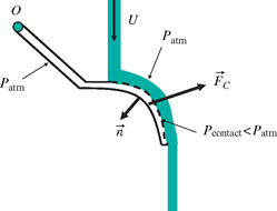
The concept of centrifugal force lies behind this notion. This effect can be demonstrated simply by placing the back of a scoop in the jet of an open tap (Figure 2.3). Due to the curvature of the scoop, the pressure decreases inside the jet following a line directed radially along ![]() . Since atmospheric pressure prevails at the water-air interface, the pressure at the contact surface between the liquid and the scoop (dashed line) is lower than the atmospheric pressure. The integral of pressure forces acting on the scoop generates a force,
. Since atmospheric pressure prevails at the water-air interface, the pressure at the contact surface between the liquid and the scoop (dashed line) is lower than the atmospheric pressure. The integral of pressure forces acting on the scoop generates a force, ![]() , since the atmospheric pressure applies on the periphery of the scoop, except for the dashed-line liquid/scoop contact surface where the pressure is lower. If the scoop is held rotatably by an axis going through O, force
, since the atmospheric pressure applies on the periphery of the scoop, except for the dashed-line liquid/scoop contact surface where the pressure is lower. If the scoop is held rotatably by an axis going through O, force ![]() reduces the torque that needs to be applied in order to maintain the inclination of the scoop in the gravity field. The pressure gradient is proportional to the squared velocity (equation [2.8]). This effect can be felt manually if the jet flows sufficiently fast and the radius of curvature of the scoop is sufficiently small.
reduces the torque that needs to be applied in order to maintain the inclination of the scoop in the gravity field. The pressure gradient is proportional to the squared velocity (equation [2.8]). This effect can be felt manually if the jet flows sufficiently fast and the radius of curvature of the scoop is sufficiently small.
In the presence of gravity: hydrostatic pressure distribution in a parallel flow
Considering the case where gravity is taken into account, it is assumed that the movement occurs in a vertical plane containing the Oz axis. For a parallel flow, R = ∞, therefore equation [2.4b] becomes:
[2.9] ![]()
Figure 2.4. Representation of the intrinsic coordinate system in the vicinity of a point around which the flow is parallel
Let us consider a point M’ in the vicinity of M, as depicted in Figure 2.4. Denoting with t and n its coordinates in the intrinsic coordinate system (![]() ,
, ![]() ), it can be written as:
), it can be written as:
[2.10] ![]()
Using the notation z for the coordinate of M’ along the gravity axis, ![]() , it can also be written as:
, it can also be written as:
[2.11] ![]()
The dot products (![]() ·
·![]() ) and (
) and (![]() ·
·![]() ) are the cosines of the angles between
) are the cosines of the angles between ![]() and
and ![]() and between
and between ![]() and
and ![]() , respectively. Since the direction of the flow is known and the flow is parallel, the unit vectors of the intrinsic coordinate system
, respectively. Since the direction of the flow is known and the flow is parallel, the unit vectors of the intrinsic coordinate system ![]() and
and ![]() at M are the same as the ones at M’, the angles are identical at any point near M, and consequently, it can be written as:
at M are the same as the ones at M’, the angles are identical at any point near M, and consequently, it can be written as:
[2.12] ![]()
equation [2.9] is therefore transformed into:
[2.13] ![]()
This equation can be integrated in any plane that is perpendicular to the direction of the flow, yielding:
[2.14] ![]()
for two points M and M’ located in the same plane SM perpendicular to the direction of the flow. The constant of integration is the pressure at M. Relation [2.14] makes it possible to determine the pressure at any point in plane SM if the pressure at a point within that plane is known. This property is very useful and will be frequently referred to. It enables the determination of the pressure field at any point in a parallel flow.
Relation [2.14] means that, for a parallel flow, the pressure variation is hydrostatic in any plane perpendicular to the direction of the flow. This property has already been highlighted for a Poiseuille flow within the gravity field (Chapter 1, section 1.7). It can be seen here that this property is much more general.
2.4. Momentum theorem
Consider a domain, D, bounded by a closed surface, S (Figure 2.5). Some portions of the surface, denoted by Ss, are solid walls, which do not permit fluid flow and the velocity of the fluid must be parallel to the wall. Other portions of the surface Sd are virtual surfaces within the fluid, which may allow flow through them. At any point M on surface S, the vector ![]() is the normal vector to surface S oriented toward the outside of the domain.
is the normal vector to surface S oriented toward the outside of the domain.
Figure 2.5. Momentum theorem. Definition of a closed volume, D, of its envelope having solid surfaces Ss (solid lines) and throughflow surfaces Sd (dashed lines), and of the normal oriented toward the outside of the domain
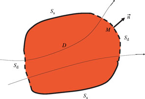
To explain the momentum theorem, it is assumed that the flow is steady and this is the only necessary assumption. It is by no means necessary for the fluid to be ideal, or even for the fluid’s rheology to be Newtonian.3
The momentum theorem is established by integrating the local equations of motion on domain D, given in Chapter 1, which are written so as to exhibit the stress deviator, Σ’ (the fluid is not necessarily Newtonian). We then obtain:
[2.15] ![]()
This expression exhibits different terms, which correspond to balances on the whole of volume D or on surface S. The term on the left-hand side is the flux (or flow rate) of momentum through surface S. This is only non-zero on the portions of surface Sd through which some flow occurs. Two contributions should be distinguished within the pressure term (the first term on the right-hand side): the integral over the throughflow surfaces Sd and that over solid surfaces Ss. On solid surfaces, we have:
[2.16] ![]()
which is the integral of the normal force exerted by the fluid on the solid wall.
The integral of body forces is the total weight of the fluid contained inside the domain, if gravity is the body force.
The integral of the stress deviator on surface S (last term in equation [2.14]) is the friction force exerted by the outside on the fluid, through the flow surfaces Sd, and on the solid surfaces Ss. In many cases, the friction force exerted through the flow surfaces is equal to zero. This is the case, for instance, when the flow is perpendicular to the throughflow surface. Here, these possible terms are neglected by writing:
[2.17] ![]()
The momentum balance can thus be written in the form:
[2.18] ![]()
Forces ![]() and
and ![]() are the global pressure and friction forces, respectively, exerted by the flow on solid walls (a minus sign appears in equation [2.17] in front of
are the global pressure and friction forces, respectively, exerted by the flow on solid walls (a minus sign appears in equation [2.17] in front of ![]() ). The left-hand side of equation [2.18] represents the impulse flux. While applying the momentum theorem, it is important to specify whether the forces under consideration are the ones exerted by the flow on solid walls or the other way round. Sign errors frequently occur when there is lack of specificity in this respect. To apply the momentum theorem, the first step is to specify domain D, throughflow surfaces Sd and solid surfaces Ss. Care must then be taken to orientate the normals in the proper direction.
). The left-hand side of equation [2.18] represents the impulse flux. While applying the momentum theorem, it is important to specify whether the forces under consideration are the ones exerted by the flow on solid walls or the other way round. Sign errors frequently occur when there is lack of specificity in this respect. To apply the momentum theorem, the first step is to specify domain D, throughflow surfaces Sd and solid surfaces Ss. Care must then be taken to orientate the normals in the proper direction.
The momentum theorem is used to answer two types of questions:
1. Evaluating the forces applied by a flow on the solid walls that surround the fluid. A classical example is the flow in a bend (see Exercise I). Section 2.5 deals with the equally classical relation between regular head loss and wall friction for the flow inside a straight pipe. In both cases, the pressure changes between the different throughflow surfaces in the domain are known.
2. Evaluating pressure drops in a flow. The classical example of a sudden expansion is presented in section 2.6. Since there is a loss of energy, Bernoulli’s theorem cannot be applied. An assumption usually enables the determination of the forces exerted by the flow on the solid walls, and the derivation therefrom of pressure changes between the inlet and outlet.
2.5. Evaluating friction for a steady-state flow in a straight pipe
Consider the flow in a straight pipe, whose walls are parallel to the Ox axis (Figure 2.6). Here, the cross-sectional geometry is arbitrary. In addition, the gravity forces are ignored and it is also assumed that the flow is unidirectional in the Ox direction. The momentum theorem applied to the closed domain bounded by the walls and the fluid inlet and outlet sections is written as:
[2.19] ![]()
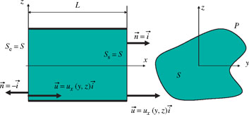
From the results of section 2.3, it can be stated that the pressure is uniform in the flow inlet and outlet sections, since the flow is parallel. Through mass conservation, the momentum fluxes between the inlet and the outlet cancel each other, as the direction of the unit normal vector is reversed between the inlet and outlet while the velocity profile is the same for both sections. We therefore deduce from equation [2.19] that:
[2.20] ![]()
The inlet and outlet throughflow sections of the pipe have an area of S. Relation [2.20] is a vector relation. The pressure force ![]() exerted by the flow on the solid side walls is perpendicular to vector
exerted by the flow on the solid side walls is perpendicular to vector ![]() , whereas the friction force,
, whereas the friction force, ![]() , is parallel to it. Consequently:
, is parallel to it. Consequently:
[2.21] ![]()
We assume that the friction stress τ exerted by the flow is uniform on the side wall. This assumption is questionable in the case of a complex cross-sectional geometry, but is wholly valid in the case of the plane Poiseuille flow or for the Poiseuille flow in a circular pipe. Therefore, it is written as:
[2.22] ![]()
where P is the perimeter of a pipe section and PL is the wetted surface of the pipe. The friction stress exerted by the flow on the sidewall is thus expressed simply as a function of the pressure gradient:
[2.23] ![]()
As can be seen, the relations obtained in Chapter 1 for Poiseuille flows are solved in equation [2.23]. For a circular pipe, S/P = R/2, hence:
[2.24] ![]()
Figure 2.7. Application of the momentum theorem on a virtual, circular cylindrical volume of radius r (shaded volume) contained within a pipe of radius R
The momentum theorem is equally applicable to any circular cylindrical volume of radius r internal to the pipe (i.e. r < R) as sketched in Figure 2.7. It then enables the calculation of the friction stress exerted by the fluid contained inside the cylinder of radius r on the fluid contained outside that cylinder. Extrapolating equation [2.24] shows that this quantity varies linearly with the radius:
[2.25] ![]()
This remarkable result holds for a laminar flow as well as a turbulent flow. Such examples illustrate the power of momentum theorem; local knowledge of the flow is not always necessary to determine wall friction. However, the pressure gradient enables its determination.
2.6. Pressure drop in a sudden expansion (Borda calculation)
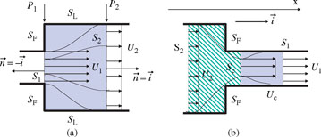
Consider the flow in a sudden expansion (Figure 2.8(a)) between two straight pipes whose walls are parallel to the Ox axis. In the expansion area, the flow is not parallel to the Ox direction. The domain to which the momentum theorem is applied (shaded domain in Figure 2.8(a)) is taken between the expansion section S1 and a downstream section S2 chosen sufficiently far away for the flow therein to become parallel again. Here, the gravity forces are ignored (the way gravity can be accounted for is discussed in section 2.7). Consequently, the pressure is uniform in sections S1 and S2, and is denoted by P1 and P2, respectively.
For a flow that is uniform in sections S1 and S2, and denoting the velocities by U1 and U2 , mass conservation is written as:
[2.26] ![]()
The momentum theorem, of which only the projection onto vector ![]() is considered here, is written as:
is considered here, is written as:
[2.27] ![]()
The pressure force on the sidewall SL has disappeared as it is perpendicular to ![]() . Force
. Force ![]() represents the pressure force on the solid wall SF, which is the end wall surrounding throughflow section S1. Borda’s model assumes that the pressure also equals P1 on SF. The pressure force
represents the pressure force on the solid wall SF, which is the end wall surrounding throughflow section S1. Borda’s model assumes that the pressure also equals P1 on SF. The pressure force ![]() is then given by:
is then given by:
[2.28] ![]()
Lastly, the friction, ![]() , exerted by the flow on the sidewall is neglected. Using mass conservation [2.26] and property [2.28], it is inferred from [2.27] that:
, exerted by the flow on the sidewall is neglected. Using mass conservation [2.26] and property [2.28], it is inferred from [2.27] that:
[2.29] ![]()
Neglecting friction can be easily justified: the distance between sections S1 and S2 is short and, consequently, the surface subjected to friction is limited. It is less straightforward to state that the pressure P1 prevails all over surface SF, due to recirculation in that zone. However, the turbulence that reigns there contributes to homogenize the pressure, which settles at the level of pressure P1 in the outlet.
Therefore, the momentum theorem makes it possible to calculate the pressure change between the inlet and outlet sections. The head change (equation [2.7]) between the inlet and outlet is then estimated (using [2.26] and [2.29]) based on the velocity in the inlet section only:
[2.30] ![]()
This model, referred to as Borda’s model, shows that the flow undergoes a loss of energy in a sudden expansion, since H1 > H2. Such dissipation is associated with the production of turbulence in the sudden expansion. Section 2.8, and further discussions in Chapter 8, explains the reasons that cause turbulence to dissipate energy.
Obviously, relation [2.30] does not hold if the direction of flow is reversed to consider the case of a sudden restriction. Otherwise, energy would need to be supplied to the flow in order to increase the head for the fluid particles. The situation of the flow in a sudden restriction is depicted schematically in Figure 2.8(b). The flow separates on the right angle of the restricted section’s inlet edge. At first, it goes through a narrowed-down section of area Sc < S1, then it spreads out. If the area Sc of the separation zone is known, mass conservation makes it possible to infer the velocity Uc, in the restriction. In the hatched zone corresponding to the restriction, the particles maintain their energy. Bernoulli’s theorem, applied between sections S2 and Sc, provides the pressure in the contracted section. Lastly, the momentum theorem, applied to the hatched domain, provides an estimate of the force applied by the flow on the end wall SF. The head loss occurs within the shaded part in Figure 2.8(b), reverting to Borda’s calculation described earlier and applying it to the expansion between Sc and S1. The unknown needed to complete the calculations is the surface, Sc, of the contracted section. Calculation rules based on experimental data, for computing head losses in many expansion and restriction situations, can be found in the well-known handbook by Idel’Cik.4
The examples presented in the last two sections show that Bernoulli’s theorem and the momentum theorem cannot always be applied simultaneously. When the momentum theorem is applied assuming that the pressures on the throughflow surfaces surrounding the domain considered are known, the forces on the walls can be deduced therefrom (as in section 2.5). When the forces are assumed known, the momentum theorem makes it possible to calculate the pressure change between the inlet and outlet sections and to deduce the pressure drop therefrom. Energy is not always conserved, as seen in the case of sudden expansion.
2.7. Using the momentum theorem in the presence of gravity
The momentum theorem is written in equation [2.18] by exhibiting the body force, ![]() . The pressure to be considered in calculating the impulse flux (left-handside term in equation [2.18]) is then the absolute pressure. The calculation of integrals is typically not straightforward because the pressure varies with height due to the effect of gravity. To circumvent this difficulty without neglecting gravity, the impulse flux integrals are calculated using pressure p’, which is equal to the difference between the absolute pressure and the hydrostatic pressure, phyd.
. The pressure to be considered in calculating the impulse flux (left-handside term in equation [2.18]) is then the absolute pressure. The calculation of integrals is typically not straightforward because the pressure varies with height due to the effect of gravity. To circumvent this difficulty without neglecting gravity, the impulse flux integrals are calculated using pressure p’, which is equal to the difference between the absolute pressure and the hydrostatic pressure, phyd.
[2.31] ![]()
The hydrostatic pressure, introduced in Chapter 1 (equation [1.36]), is written as:
[2.32] ![]()
where p0 is a reference pressure taken at point O. Pressure p’ is homogeneous in throughflow sections Sd if the flow is perpendicular to the throughflow section (see section 2.3), and the calculation of integrals poses no further difficulty. This very simple procedure enables a rigorous application of the momentum theorem in the presence of gravity, by omitting the gravity force in equation [2.18] of the momentum theorem.
2.8. Kinetic energy balance and dissipation
It is seen that a sudden expansion (Figure 2.8(a)) results in energy dissipation: the head decreases between the inlet and the outlet (equation [2.30]). The rate of energy dissipation evaluates how fast the kinetic energy is dissipated. For the sudden expansion, it is possible to estimate an average rate of kinetic energy dissipation per unit mass, ![]() , by computing the ratio of the head change to the time of residence in the sudden expansion, namely:
, by computing the ratio of the head change to the time of residence in the sudden expansion, namely:
[2.33] ![]()
This formula involves the flow rate and the volume of the sudden expansion.
In reality, the rate of dissipation is a local physical notion that varies in both space and time. As will be seen hereinafter, turbulence dramatically increases the rate of energy dissipation, and hence its paramount importance in fluid mechanics. The rate of energy dissipation can be defined rigorously on the basis of the Navier– Stokes equations, by establishing the evolution equation for kinetic energy. For this derivation, it is assumed that the fluid is incompressible.5 A tensor notation is used (Einstein’s notation) where the velocity vector is expressed in the form ui, with index i varying from 1 to 3 to designate the three space dimensions (namely u1 = ux, u2 = uy and u3 = uz). The local equations can then be written as:
for incompressibility
[2.34] ![]()
for the equations of dynamics
[2.35] ![]()
While the tensor notation is convenient for subsequent calculations, it should be remembered that, in equations [2.34] and [2.35], the terms involving index j are summed for all three values of j, i.e. in equation [2.35],
There are also three equations of dynamics for each value of index i = 1, 2, and 3. Equations [2.35] are written using the symbolic notation of the stress deviator, to simplify intermediate calculations. The expression of the stress tensor for a Newtonian fluid will be used later on.
By multiplying each of the equations [2.35] of dynamics by ui, respectively, three equations are obtained for i = 1, 2, and 3.
Summing these three equations over index i brings in the kinetic energy per unit volume:
[2.37] ![]()
whose evolution equation is:
[2.38] ![]()
Equations [2.37] and [2.38], and the subsequent ones, are now summed over indices i and j.
Differentiation formulae yield some simplifications, thanks to incompressibility:
[2.39] 
Evolution equation [2.38] for kinetic energy therefore becomes:
[2.40] ![]()
that is:
[2.41] ![]()
This formulation, which brings in the divergence of certain vectors, is attractive because, by integrating the equation over a volume D, it is possible, through Ostrogradsky’s formula, to transform the volume integrals in some of the terms into integrals over surface S, which surrounds volume D. This results in the appearance of flux terms through surface S. These transformations lead to:
[2.42] ![]()
Finally, the symmetry of the stress tensor yields:
[2.43] ![]()
The physical meaning of the different terms is worthy of some clarifications. From left to right, it is encountered in sequence:
– The rate of variation of the kinetic energy contained in the volume.
– The head flux through the surface surrounding the domain. Gravity forces may be incorporated into this term, through potential energy.
– The power of friction stresses at the boundaries.
– The rate of energy dissipation.
Now, specific attention is given to the fourth term, i.e. the rate of energy dissipation. For a Newtonian fluid, bringing the expression of the stress deviator tensor (Chapter 1, Table 1.1) in, the rate of energy dissipation, integrated over the volume, can be written as:
[2.44] ![]()
since the summation takes place on both i and j indices. As a result, we arrive at the following conclusions:
– This quantity is always negative. Therefore, it is justified in referring to it as the rate of dissipation of kinetic energy, as it can only contribute to decrease kinetic energy.
– Energy dissipation is linked to velocity gradients. The larger the velocity gradients in the flow, the stronger the dissipation. It can therefore be anticipated that dissipation will be very large in a turbulent flow. The kinetic energy dissipated is thereby turned into heat. For fluids such as water or air, the warming induced by dissipation is very weak (see Exercise III at the end of this chapter). But for highly viscous fluids in configurations where the flow is strongly sheared, such as a liquid polymer in an extruder, the amount of self-heating resulting from viscous dissipation can be very large.
– The dissipation rate per unit mass, denoted by ε, can thus be defined as a local quantity by:
[2.45] ![]()
The spatial distribution of this quantity is typically highly inhomogeneous. These aspects will be explained in Chapter 8, while dealing with the concepts of turbulence.
2.9. Application exercises
The exercises proposed below are applications of Bernoulli’s theorem and the momentum theorem. As demonstrated in this chapter, these two theorems cannot always be applied simultaneously, because applying Bernoulli’s theorem implies energy conservation, whereas energy is obviously not conserved if the momentum theorem is used to estimate a head loss. The first challenge is to know when and in which regions of a flow it can be considered that energy is conserved, and when the flow is dissipating energy. This will be explained in Chapter 4. The wording of the following exercises is deliberately kept somewhat ambiguous, because if it is indicated which of Bernoulli’s theorem or the momentum theorem should be applied (specifying in which domain) there would no longer be an exercise to solve, but only calculations to perform.
Exercises 2.I–2.III and 2.V are classical ones. Exercise 2.IV compares the results of a local approach to those yielded by the global approach, establishing a link with Chapter 1. Exercises 2.VI and 2.VII are more complex. In those cases, the flow does not dissipate energy in certain subdomains, while in others it dissipates some. Based on Borda’s model, it will be assumed that energy is conserved in regions where the flow is convergent (the available cross section diminishes) and that dissipation occurs in domains where a sudden expansion occurs.
Exercise 2.I: Force exerted on a bend
A circular cylindrical pipe whose diameter is 50 cm goes through a 90° bend. If the water flow rate in the pipe is 1 m3 s−1, calculate the force applied by the flow onto the support (orientation and magnitude). The absolute pressure measured at the inlet of the bend is 2 bar and the air surrounding the pipe is assumed to be at a pressure of 1 bar.
Carry out the numerical application and discuss the way in which the ambient atmospheric pressure should be taken into account.
Exercise 2.II: Emptying a tank
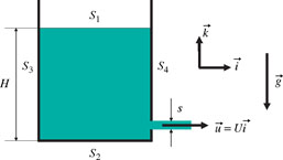
Here, we analyze what can be learnt from the application of the Bernoulli’s and momentum theorems when they are applied to the emptying of a tank in which the water level is H.
1. Establish Torricelli’s formula, which gives the velocity of the fluid at its exit from the tank. For this question, it will be assumed that the pressure in the jet is the atmospheric pressure.
2. Using the results from section 2.3, explain which effect allows the pressure (within the gravity field) to actually settle at the atmospheric pressure in the jet at the tank outlet.
3. Calculate the force exerted on the walls of the tank. How would the tank behave if it was mounted on wheels and able to roll without friction?
Figure 2.II.1
Exercise 2.III: Pressure drop in a sudden expansion and heating
Consider a sudden expansion such that S1 / S2 =1/ 3 . The inlet velocity is 5ms−1.
Determine:
– The head loss;
– The temperature rise;
The numerical application will be carried out with water as the fluid (mass density ρ = 103 kg m−3, specific heat Cp = 4.2 103 J kg−1 K−1).
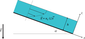
Exercise 2.IV: Streaming flow on an inclined plane
Consider the streaming flow on an inclined plane lying at an angle α to the horizontal plane (imagine a river). Gravity is along the vertical axis. In a uniform flow regime, the thickness h of the fluid layer is invariant. It does not depend on coordinate x in the coordinate system indicated in the Figure 2.IV.1. The flow is assumed to be two-dimensional (that is, ux(x, z)) and unidirectional (uy = uz = 0). ρ is the mass density of the fluid, and μ its dynamic viscosity.
Figure 2.IV.1
Part 1 – Do not use the local solution of the Navier–Stokes equations
1.Why is the ux velocity component independent from x?
2.Determine the pressure field.
3.Determine the head at every point in the liquid. Which term causes the head loss in the flow along a streamline?
4.Determine the friction stress exerted by the flow on the solid wall.
Part 2 – Use of the Navier–Stokes equations
1. Write out the Navier–Stokes equation for the ux velocity component (along Ox), using the assumptions made about the kinematics of the flow and the results established in the first part?
2. Write out the boundary conditions on the bottom (z = 0) and at the free surface (z = h).
3. Determine the velocity profile, ux(z)?
4. Calculate the friction stress exerted on the bottom by the flow, using a method other than the one used in Question 4 of Part 1?
5. Calculate height h as a function of the flow rate Q injected by unit width?
Exercise 2.V: Impact of a jet on a sloping plate
Consider, in a two-dimensional configuration, a jet of water that impinges on a flat plate defining an angle α with the direction of the incident flow (the jet impinges perpendicularly on the plate when α = π/2). The upstream thickness of the jet is denoted by e and the thicknesses along the plate on either side of the incident jet’s axis are denoted by e1 and e2. Besides the pressure of the gaseous atmosphere is denoted by po, which is also exerted on the rear side of the plate. The velocity in the incident jet is assumed to be uniform, which is denoted by U. At a sufficient distance from the incident jet’s axis, velocities are also assumed to be uniform in the throughflow sections, and are denoted by U1 and U2.
Figure 2.V.1
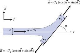
1. Determine:
2. If it was now assumed that the fluid particles undergo a head loss on impact, would thicknesses e1 and e2 be greater or smaller than the ones obtained in Question 1?
Exercise 2.VI: Operation of a hydro-ejector
This exercise aims to understand the principle of operation of a hydro-ejector, which is an apparatus used, for example, for cleaning the walls of a basin.
Part I – Jet from a submerged pump
In the first stage, we consider a simplified configuration where the apparatus simply consists of a submerged pump, which draws water from inside the basin and discharges it in the same basin in the form of a jet. The suction and discharge pipes are circular cylindrical pipes, which have the same diameter, D0 = 0.1 m. Velocity Uj is assumed to be uniform at the outlet of the discharge line (Figure 2.VI.1). The axis of the apparatus is horizontal within the gravity field.
The characteristic of the pump is plotted in Figure 2.VI.2. The head/velocity relationship can be represented by a parabolic function
![]()
with numerical values Pmax = 105 Pa and α = 9.
Figure 2.VI.1
Figure 2.VI.2
1. State the operating conditions of the pump in terms of flow rate and head.
2. What is the momentum flux discharged by the apparatus?
Part II – The hydro-ejector
Figure 2.VI.3
To form a hydro-ejector (Figure 2.VI.3), the jet produced by the apparatus considered in part I is fed into a tube with diameter D1 = 0.2 m, allowing a secondary supply by entrainment. In plane P, it is assumed that the jet produced by the primary supply (velocity Uj) is always uniform with 0 < r < D0/2; the same is true of the velocity Ue of the secondary feed with D0/2 < r < D1/2 in plane P. At the outlet of the hydro-ejector (plane P’), the velocity is assumed to be homogeneous, which is denoted by U. The length of the tube is not a parameter of the problem. It is assumed sufficiently large to allow the velocity field to become homogeneous, and sufficiently short to allow wall friction to be neglected.
For simplicity, it is assumed that the velocity Uj is the same as the one determined in Question 1. If Question 1 has not been solved, a value of Uj = 4 ms−1 may be used. The pressure value, however, is not necessarily the same. The axis of the hydro-ejector is located at a depth h under the free-surface level of the basin.
3.What indications can be provided regarding the pressure field in planes P and P’? (Numerical values will be calculated at the end of Question 5.)
4.Explain the mechanism that draws fluid through the secondary supply. State a first relation involving Ue.
5. Calculate the entrainment velocity Ue, the velocity U at the outlet of the hydro-ejector, and the numerical values of the pressure. Calculations will be facilitated by bringing in the ratio of the area of the primary jet to that of the hydroejector tube, s = D02/D12 = 1/4, as well as the velocity ratio, Uj/Ue.
6. What is the power consumption of the hydro-ejector? Compare this to an equivalent estimate that can be derived for the apparatus considered in part I.
7. Calculate the flow rate of the hydro-ejector, as well as the rate of momentum at the outlet of the hydro-ejector (plane P’). Explain one benefit of the hydro-ejector by comparing it to the configuration without a secondary supply tube as studied in part I.
Exercise 2.VII: Bypass flow
This exercise is inspired by cooling problems in an industrial facility. Part of the flow of a river is diverted and fed into a bypass channel that goes through a grid with which it exchanges heat. The exercise deals with the hydraulics problem: how is the flow rate distributed between the bypass channel and the river?
Figure 2.VII.1
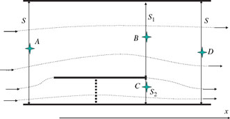
For the solution of this problem, gravity will not be considered. The fluid is water. For simplicity, it is assumed that the channels are rectilinear in geometry, as shown in the Figure 2.VII.1, and wall friction is neglected. The grid induces a singular head loss in the flow, written as ΔH = KpU22 /2. K = 3 will be used for the numerical applications.
We denote by U = 1 m s−1, U2 and U1, respectively, the velocities in the inlet section (whose area is S = 1,000 m2) containing points, in the outlet section of the bypass channel (area S2 = 200 m2) containing point C, and in the outlet section of the other channel (area S1= 800 m2) containing point B. The velocity is assumed to be uniform in all the sections considered. The pressure at A is PA = 1 bar.
1. Justify why the pressure is the same at B and C.
2. By considering energy conservation (or non-conservation) between A and B, then between A and C, determine velocities U2 and U1. Deduce therefrom the difference in pressure, PA – PB, between points A and B.
3. It is assumed that the fluids are again completely mixed in the outlet section containing point D. Explain why the head cannot be conserved between B and D. By applying the momentum theorem on a domain to be specified, calculate the pressure difference, PB – PD, between points B and D.
1 Here, we simplify the case of a flow within a plane.
2 The term “head” often refers to the quantity H/ρg, which is homogeneous to a length. This quantity is conveniently used when pressure changes are measured as water heights. Our definition is closer to the notion of energy. Either of these can be used, provided that consistency is maintained throughout.
3 Exercise I in Chapter 7 uses the momentum theorem for a Bingham fluid.
4 I.E. Idel’Cik, 1960, Mémento des pertes de charge (translated from Russian), Editions Eyrolles, Paris.
5 The following discussion is much inspired by section 16 of the book of L.D. Landau and E.M. Lifshitz, Fluid Mechanics (2nd Edition, Butterworth-Heinemann, 1987), which is outstandingly clear.