11
Network Planning
Brian Olsen, Pablo Tapia, Jussi Reunanen, and Harri Holma
11.1 Introduction
The proper planning of the HSPA+ is a very important activity that will determine to a large extent the coverage, capacity, and quality of the service. No matter how much effort is invested in maintaining a network, if the original planning is flawed it will be a constant headache for the engineering teams.
The main focus area when deploying HSPA+ are the radio nodes, including NodeB site location and antenna and power configuration. This chapter provides practical guidelines to take into account when performing the RF planning, however it does not include the amount of detail that can be found in specialized RF planning books such as [1]. Although the main emphasis is put on the Radio Access Network (RAN) nodes, basic considerations around core and backhaul design are also discussed.
In addition to deployment aspects, the chapter also provides useful information to help manage capacity growth, including multilayer management and network dimensioning guidelines.
11.2 Radio Frequency Planning
The performance at the radio layer has a direct impact on the experienced data rates on the application layer and, ultimately, on the experienced user data rate at the application layer. The stronger and cleaner the signal, the higher the data rate that can be achieved; and vice versa, in challenging radio conditions the throughput will be reduced since the physical layer adapts the Modulation and Transport Format to avoid excessive packet loss. The radio signal is typically measured in terms of Received Signal Code Power (RSCP) and interference levels: Energy per chip over Interference and Noise (Ec/No) for downlink and Received Signal Strength Indicator (RSSI) for uplink.
The main challenge when planning the radio network is to do so considering both coverage and interference performance, with consideration for future traffic growth. HSPA+ systems utilize a single frequency reuse, which means that the same frequency is used in all adjacent sectors and therefore is highly susceptible to interference. Many of the problems found in today's networks can be tracked down to poor Radio Frequency (RF) planning. In many cases, the problems are masked by adding additional capacity or new sites to the network, but they will eventually need to be addressed through proper optimization.
The placement and orientation of the antenna is the best tool the operator has to ensure proper RF planning, therefore this activity should be done very carefully. To help with this task it is advisable to use network engineering tools like RF Planning and Automatic Cell Planning (ACP) tools, which will be covered in Section 11.2.3.
When configuring antenna parameters, the operator needs to strike a balance between coverage and capacity. When a technology is first deployed, the network needs to provide service in as many locations as possible, so coverage will normally be the initial driver. Ensuring a good level of coverage with HSPA+ can be quite challenging, especially when evolving the network from a previous GSM layout, since in UMTS/HSPA+ it is not possible to use overlay (boomer) sites. Having sectors inside the coverage area of other sectors is very harmful due to the single frequency reuse nature of the technology. Contrary to common wisdom, in some cases, the coverage versus interference tradeoff will result in the reduction of transmit powers, or even the deactivation of certain sectors.
A second challenge when building a coverage layer is deciding the transmit power to be used. In dense urban areas, having too much signal strength beyond a certain point can actually hurt the network performance. The reason is that signals will propagate outside of the desired coverage zone and interfere with sectors in other places – this in turn may create the sensation of a “coverage hole” when in reality the problem is that the network is transmitting with too much power.
Along the same lines, UMTS networks experience so-called “cell breathing” when the network gets loaded, which shrinks the effective coverage of the sectors due to an increase of interference at the cell borders. The “more power is better” guiding principle doesn't always apply, and often ends up causing significant performance degradation as network traffic grows. This is why it's important to try and design the network for a certain load target, for example 50%. To do this in practice the operator should use realistic traffic maps during the planning stage.
Achieving pilot dominance is very important for the long-term health of the network. Well defined cell boundaries will minimize problems related to pilot pollution and will enable a more gracious cell breathing as the network gets loaded. Figure 11.1 illustrates a network in which the original RF configuration (a) has been optimized to minimize interference in the area (b). As the maps show, the optimized network has clearer sector boundaries, although these are still far from perfect in some areas given the challenges from the underlying terrain.
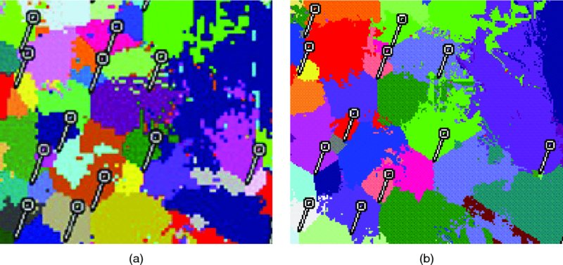
Figure 11.1 Example of poorly defined boundary areas (a) and optimized boundaries (b) in the same network
Considering that every network is different, the operator needs to make the appropriate decisions taking into account the terrain, the frequency bands in use (low bands are more prone to interference, high bands are more challenged in coverage), and the antenna configuration, among other issues. Since typically UMTS networks are uplink limited – both from coverage and interference points of view – one good idea is to explore the option to have additional receive antennas and enable the 4-Way Receive Diversity feature in the NodeB. This feature can significantly improve uplink performance, as was discussed in Chapter 10.
In summary, below are a few guidelines to UMTS radio planning:
- Deploy based on traffic location: the closer the cell is to the traffic source, the lower the interference introduced in the system, and the more efficient the air interface will be.
- Proper definition of cell boundaries, avoiding zones with pilot pollution by creating a dominant sector in each particular area.
- Limit footprint of sectors: avoid overshooting sectors that can capture traffic outside their natural range. By the same token, do not abuse antenna downtilts, which are often used as the only method to achieve interference containment and can create sudden attenuation areas within the cell footprint.
- Do not use excess power, try to serve the cell with the minimum power required to keep the service at the desired quality level – taking into consideration service coverage inside buildings.
- In case of overlaid GSM deployment, identify and correct harmful inherited configurations such as boomer sites, sectors that are pointing at each other, and unnecessary capacity sites.
11.2.1 Link Budget
The first step toward planning the radio network is to perform an estimation of the coverage area that the technology can provide. While this is a complicated exercise that needs to consider many different factors, a first order approximation is to analyze the maximum pathloss that can be endured both in the uplink and downlink directions to achieve a certain level of quality. This is known as link budget calculation. This section will provide useful guidelines to help calculate the link budget for HSDPA and HSUPA, however more detailed explanation on computing link budget can be found in network planning books such as [1].
At a very high level, the link budget exercise will estimate the maximum pathloss permitted to transmit with a given quality; there will be many factors affecting the link budget, such as technology, network configuration, type of data service, network load, and interference conditions. The link budget calculations for uplink and downlink are quite different, given the different nature of the service: while HSUPA is transmitted over a dedicated channel that is power controlled, the HSDPA service is carried over a shared channel whose power is determined based on operator configuration and load demands.
In practice, HSPA+ networks are UL coverage limited. Therefore, the first step to compute the link budget would be to estimate the cell range based on the required UL speed, and afterwards calculate the corresponding DL bitrate for that particular pathloss.
The following steps describe the generic process used to estimate the link budget on the uplink direction:
- Determine required bitrate at cell edge.
- Estimate required signal quality for such bitrate (Eb/Nt). This is provided by link level simulations – sample mapping values can be found in [2].
- Compute UE Equivalent Isotropical Radiated Power (EIRP) considering UE Max Transmit power and a HSUPA back-off factor. Back-off factors for commercial power amplifiers range from 2.5 dB for smaller bitrates, up to 0.5 dB for the higher bitrates.
- Estimate the minimum required power at the BTS to receive the transmission at the given bitrate (receive sensitivity):
- calculate the noise floor of the system;
- calculate UL noise rise based on target system load;
- calculate the processing gain based on the target bitrate required;
- estimate the UL noise increase in the cell when the UE will be transmitting at the required bitrate;
- compute the sensitivity considering all previous calculations.
- Estimate the difference between the UE EIRP and the required sensitivity, considering adjustment factors such as:
- BTS antenna gain and cable losses;
- fading margin;
- soft handover gains.
Table 11.1 illustrates an example calculation for a network with a target 50% load.
Table 11.1 Example HSUPA outdoor link budgets for 64, 256, and 512 kbps at 50% load
| Target UL data rates (kbps) | ||||
| Parameters and calculations | 512 | 256 | 64 | |
| UE Tx power | UE maximum transmit power (dBm) | 21.0 | 21.0 | 21.0 |
| UE cable and other losses (dB) | 0.0 | 0.0 | 0.0 | |
| UE transmit antenna gain (dBi) | 0.0 | 0.0 | 0.0 | |
| Power back off factor (dB) | 1.1 | 1.7 | 2.3 | |
| Mobile EIRP (dBm) | 19.9 | 19.3 | 18.7 | |
| Required power at the BTS | Thermal noise density (dBm/Hz) | −174.0 | −174.0 | −174.0 |
| BTS receiver noise figure (dB) | 3.0 | 3.0 | 3.0 | |
| Thermal noise floor (dBm) | −105.2 | −105.2 | −105.2 | |
| UL target loading (%) | 50% | 50% | 50% | |
| UL noise rise (dB) | 3.0 | 3.0 | 3.0 | |
| Required Eb/Nt (dB) | 3.9 | 4.0 | 4.8 | |
| Processing gain (dB) | 8.8 | 11.8 | 17.8 | |
| Interference adjustment factor (dB) | 1.2 | 0.7 | 0.2 | |
| NodeB Rx sensitivity (dBm) | −105.7 | −109.3 | −114.9 | |
| Maximum pathloss | BTS antenna gain (dBi) | 18.0 | 18.0 | 18.0 |
| BTS Cable connector combiner losses (dB) | 4.0 | 4.0 | 4.0 | |
| Slow fading margin (dB) | −9.0 | −9.0 | −9.0 | |
| Handover gain (dB) | 3.7 | 3.7 | 3.7 | |
| BTS body loss (dB) | 0.0 | 0.0 | 0.0 | |
| Maximum allowable pathloss (dB) | 134.3 | 137.3 | 142.3 | |
The maximum pathloss values provided are calculated for outdoor transmissions; in the case of indoor, an additional in-building propagation loss should be subtracted, which is typically in the 15–20 dB range. Other adjustments should also be taken into account: for example, the use of uplink advanced receivers, or receive diversity methods that were described in Chapter 8.
Once the Maximum Allowable Pathloss (MAPL) has been determined, the HSDPA link budget exercise will estimate the downlink bitrate that is possible at that particular cell location. The following steps summarize the process:
- Determine power breakdown in the cell: overhead of control channels, power for voice, and available power for HSDPA.
- Calculate the received signal levels for the HS-DSCH channel, own cell interference, and noise:
- calculate EIRP values considering BTS antenna gains, cable and feeder losses and adjust with MAPL values;
- calculate noise floor considering thermal noise density and UE noise figure.
- Calculate the Geometry (G) factor at that particular location.
- Estimate SINR for the given G factor, and calculate the bitrate at that particular level based on pre-defined mapping tables.
The geometry factor indicates how susceptible that location is to receiving interference from external cells. It is defined as:
Where:
- Pown is the power from the serving cell.
- Pother is the interference power from the rest of the cells.
- Pnoise is the thermal noise power, No.
It is important to estimate the right geometry factor for the required scenario, as it will define whether the network is interference or coverage limited. In many cases, geometry, and not noise, will be the limiting factor in HSDPA networks. Geometry factors range from over 20 dB, for users close to the cell site, to below −5 dB, for users at the cell edge in pilot polluted areas. Typical values for cell edge in urban areas are around −3 to −4 dB.
One other important factor to consider in the HSDPA link budget exercise is the orthogonality factor(α) which takes into account the impact of multipath propagation on the Signal to Interference and Noise ratio (SINR) [3]. The orthogonality factor is 1 for non-multipath environments, such as rural areas, and 0.5 for typical environments.
The SINR will determine the achievable bitrate for the HSDPA service. In interference limited conditions, the SINR for HSDPA can be estimated as:
Where:
- SF16 is the processing gain corresponding to the spreading factor 16 (12 dB).
- PTOT_BS is the total power transmitted by the BTS.
- PHSDPA is the power available for the HS-DSCH channel.
The power allocated to the HSDPA service depends on the specific vendor implementation (static vs. dynamic allocation) and operator configuration. Nowadays, most HSDPA networks allocate the power dynamically, with a low power margin to maximize the bitrates in the sector.
Table 11.2 provides some example values for the required SINR to achieve certain downlink bitrates, based on HSDPA Release 5 [4].
Table 11.2 SINR requirement for various DL bitrates
| SINR | Throughput with 5 codes | Throughput with 10 codes | Throughput with 15 codes |
| 0 | 0.2 | 0.2 | 0.2 |
| 5 | 0.5 | 0.5 | 0.5 |
| 10 | 1.0 | 1.2 | 1.2 |
| 15 | 1.8 | 2.8 | 3.0 |
| 20 | 2.8 | 4.2 | 5.5 |
| 25 | 3.1 | 5.8 | 7.8 |
| 30 | 3.3 | 6.7 | 9.2 |
The HSDPA advanced receivers will significantly improve SINR, especially at challenging cell locations such as the ones found at cell borders in urban areas (low G factors).
Table 11.3 provides some example SINR and throughput under various network configuration and geometry factors, for a cell with a minimum HSUPA bitrate of 64 kbps (MAPL of 142 dB). The maximum BTS power is set to 20 W.
Table 11.3 Example cell edge DL bitrates for various HSDPA configuration scenarios, for MAPL = 142 dB and α = 0.5
| Configuration | G-factor (dB) | HS power (W) | SINR (dB) | DL bitrate (Mbps) |
| 1 | 14 | 12 | 12.3 | 2.0 |
| 2 | 14 | 7 | 10.0 | 1.2 |
| 3 | 0 | 7 | 5.6 | 0.6 |
| 4 | −3 | 7 | 3.5 | 0.4 |
| 5 | −3 | 12 | 5.8 | 0.6 |
These results highlight the importance of the geometry factor in the achievable HSDPA data rates. The scenario with high G factors (coverage limited) can achieve significantly higher throughputs than those with lower G factor (interference limited). This is one of the reasons why too much cell coverage overlap with HSDPA should be avoided. This also explains why assigning higher power to the cell will not be an effective method to extend the cell coverage in the case of interference limited networks. Table 11.3 also shows that increasing the power available for the HS-DSCH channel can help improve the bitrates at the cell edge; as expected, such improvement will be higher in coverage limited situations.
Table 11.4 calculates the downlink bitrates for various locations in the cell corresponding to the MAPL calculated for UL 64, 256, and 512 kbps. The network follows the configuration #4 from Table 11.3 for a network limited by interference.
Table 11.4 Calculated DL bitrates for various locations for Max HSDPA power allocated = 7 W, G factor at cell edge = −3 dB
| Pathloss (dB) | UL bitrate (kbps) | G factor (dB) | SINR (dB) | DL bitrate (Mbps) |
| 142 | 64 | −3 | 3.5 | 0.4 |
| 137 | 256 | 7 | 9.0 | 0.9 |
| 134 | 512 | 13 | 12.2 | 2.0 |
11.2.2 Antenna and Power Planning
Selecting the right antenna for a site is just as important as selecting the right tires for a car. Like tires, they are small part of the overall site cost, but they are often overlooked even though they have a tremendous impact on achieving the desired coverage and capacity performance.
Some of the most common antenna characteristics are the peak antenna gain and horizontal 3 dB beamwidth, however they shouldn't be the only ones considered when evaluating antenna selection for a site. The antenna's vertical 3 dB beamwidth, which is inversely proportional to the peak main lobe gain, is just as important. Other important considerations are the front-to-back ratio, front-to-side ratio, and the power of the 2nd and 3rd sidelobes relative to the mainlobe. Figure 11.2 illustrates some of these parameters.
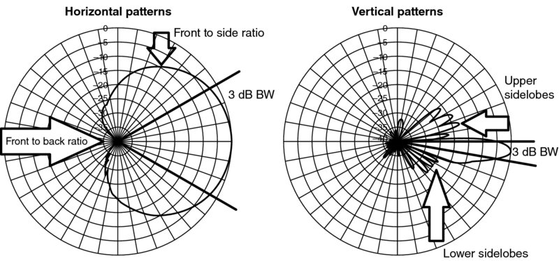
Figure 11.2 Example horizontal and vertical antenna patterns
The antenna packaging and radome are also important considerations. As more physical antennas are packaged into the same radome (i.e., Dual POL and Quad POL) there is a tradeoff made in the shape of the antenna pattern. The peak antenna gain is often used as the most important figure of merit, but the intended geographical area the antenna is attempting to serve is just as important. So ideally the antenna shape should match the intended coverage in all three space dimensions. As an extreme example, an antenna on a mountaintop with a high gain and small vertical beamwidth may appear to provide the best signal strength over a large geographical area on a two-dimensional propagation prediction, but in practice there may actually be coverage holes closer to the sites because the coverage is being provided by the lower sidelobe of the vertical pattern where there may be nulls in the pattern that are not very well behaved. In this situation it is often better to use an antenna with a larger vertical beamwidth and less peak gain so that the antenna pattern does not contain any nulls or large changes in gain toward the intended coverage area.
There are often practical limitations regarding which antennas should be utilized as often in mature networks antennas are shared between multiple technologies as discussed in Section 11.6.4. In many cases, the operator may need to transmit in multiple bands, for which it is possible to use multiband antennas. These antennas can operate in a large range (700–2600 MHz) and present a pretty good performance, which makes them a good choice for future capacity growth as well as carrier aggregation scenarios.
Antenna sharing may limit optimization such as azimuth, tilt, or height adjustments on a per band/technology basis, so a compromise must be struck in antenna design that may not be optimal for either technology as each technology on a site may not share the exact same coverage objectives. Other practical aspects may limit the adjustment of the ACL (Antenna Center Line) height. For example, sites located on high-rise rooftops may not have the ability to lower the ACL as the network densifies and the coverage objectives for a site are reduced, so downtilt and reductions in the transmit power may need to be utilized to optimize the coverage. However, as antenna downtilts are deployed, care must be taken not to place any nulls of the antenna pattern toward the intended coverage area.
The goal of the RF design is to ensure that the “well behaved” portion of the antenna is pointed at the intended coverage area. Often, antenna adjustments such as downtilt are over-used and the top portion of the vertical antenna pattern, which can have high variations in gain, is used to serve the coverage area leading to large drops in signal strength over the sectors intended coverage footprint. In an attempt to create a “dominant” coverage area the excessive downtilt can create significant coverage issues, which can become especially evident in sectors with low antenna height. Consider Figure 11.3, which illustrates the typical antenna range of a rooftop antenna in a suburban neighborhood (around 10 m height). Figure 11.3b shows the 2D pattern of an antenna with 6° vertical beamwidth that is downtilted by 6°.

Figure 11.3 Effect of excessive antenna tilt on footprint (a) and antenna pattern (b)
In the case of low antenna height, downtilting by 6 degrees or more pretty much points the main lobe of the antenna confines to less than 100 meters next to the sites; furthermore, considering the practical effects of real antenna patterns, the boundary area of the sector will be exposed to unpredicted attenuation that can change every few meters, due to the steep slope of the antenna pattern around the beamwidth zone. This often results in the creation of very hot areas next to the antenna, and artificially attenuated signal strength and signal quality inside the sector footprint leading to undesirable spotty coverage holes in between neighboring sites. The antenna pattern gain is reciprocal for the uplink and downlink, so the excessive downtilt impact is especially harmful to the uplink as it is the limiting link in terms of coverage. Since cell selection is controlled by the downlink coverage of the pilot, a more effective way to control the coverage footprint without negatively affecting the uplink is to adjust the pilot power.
The pilot power should be utilized to cover the intended coverage objective; however, as the pilot power is reduced the overall power of the Power Amplifier (PA) must be reduced by the same ratio in order to maintain the proper Ec/No quality. A typical rule of thumb is to ensure that the CPICH power is between 8 and 10% of the max power of a carrier and that the overhead power for control channels doesn't exceed 25% of the max carrier power. The recommend CPICH power will place the transmit Ec/No of a carrier at −10 to −11 dB when the entire power of the carrier is fully utilized at maximum load. Using a lower ratio risks eroding the Ec/No quality, which will limit the sector coverage area. Using a higher ratio will increase the sector coverage at the expense of less total power available for customer traffic, which may limit the overall sector capacity.
As additional sites are added and the network becomes more dense care must be taken to review the coverage of the neighboring sites and to make adjustments so that sites are not just integrated in terms of neighbor list optimization, which might mask interference problems, but to incorporate new coverage objectives for all the neighboring sites.
As the network densification continues and new coverage and capacity objects are introduced, the intended coverage of each site will need to be optimized holistically. These changes can include small things such as antenna changes, tilt adjustments, azimuth changes, and transmit power reductions. However, over time more drastic changes, such as lowering the height of a site, deactivating sectors or an entire site that are no longer needed from a coverage and capacity perspective, may be required as a network densifies and matures. As the inter-site distance in a dense network decreases, the effective antenna height and transmit power will need to be reduced accordingly so that the capacity of the network can continue to increase and inter-cell interference is reduced. As this process continues in the dense portions of a network over time the distinction between classic macro cell networks and low power micro cell networks begins to blur.
11.2.3 Automatic Cell Planning (ACP) Tools
Automatic Cell Planning (ACP) tools can be of great help with the RF planning and ongoing optimization of the HSPA+ networks. These tools compute multiple combinations of RF parameters, typically based on a heuristic engine embedded within a Monte Carlo simulator, to come up with an optimized configuration, including:
- optimum location of the sites based on a set of predefined locations;
- height of the antennas;
- azimuth orientations of the sector antennas;
- antenna downtilts (mechanical and electrical);
- pilot powers.
The accuracy of the results of the ACP tool depends to a large extent on the input data supplied. Given that traffic is not uniformly distributed in real networks, it is recommended to utilize geolocated traffic maps. Ideally this information will be provided from a geolocation tool such as those discussed in Chapter 12; however, this can also be achieved through configuration of typical clutter maps. Geolocation information can also be used to tune the propagation maps used in the ACP exercise; otherwise the tool can be tuned with drive test data to complement the input from the prediction engine.
The following example shows the result of an ACP optimization on a live HSPA+ network. The original network was experiencing quite challenging radio conditions, both in terms of signal strength (RSCP) and quality (Ec/Io). In the exercise, the tool was configured to only modify electrical tilts, and the optimization targets were set to RSCP = −84 dBm and Ec/Io = −7 dB.
Figure 11.4 illustrates the modification of antenna tilts in the network. The original tilts are on the left, and the optimized settings on the right. In this particular case a large number of antennas were uptilted, shifting the median tilt value from 7 to 4 degrees.
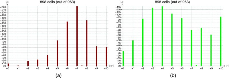
Figure 11.4 Baseline (a) and recommended antenna tilts (b)
As a result of the tilt changes, the RSCP in the region improved significantly: the number of customers served with RSCP higher than −87 dBm increased from 65 to 85%. Furthermore, with the new settings, the whole area was covered at a level higher than −102 dBm, while previously only 85% of the population was at this level. The quality in the area was also significantly improved, as can be appreciated in Figure 11.5. The results of this test indicate that the network was coverage limited, and the excessive downtilt was making the problem worse.

Figure 11.5 Ec/No improvement after ACP execution. Baseline (a), Optimized (b)
After the implementation of the ACP proposed changes, the operator should closely monitor the performance in the cluster. If a geolocation tool is not available, it is recommended to perform a thorough drive test in the area where new changes have been made and compare the main RF metrics against the results predicted by the ACP tool.
Once the network carries a significant amount of traffic, it will be possible to perform these optimization exercises automatically with the use of a Self-Organizing Networks (SON) tool. These tools are discussed in Chapter 12 (Network Optimization).
11.2.4 Neighbor Planning
The configuration of neighbors is a very important task in a HSPA+ system since cell footprints can be very dynamic due to traffic growth and the deployment of new sites for coverage or capacity purposes. Furthermore, due to the single frequency reuse, neighbors that are not properly defined will be a direct source of interference to the devices when they operate in overlapping areas.
Neighbor management can be broken down into two main categories, the initial configuration of neighbors when a site is deployed, and a continued maintenance once the site has been put on air. This section will provide guidelines to consider for initial neighbor configuration, while Chapter 12 (Optimization) will discuss ongoing optimization aspects.
The HSPA+ cells need to be configured with three types of neighbors:
- Intra-frequency neighbors, which define the sector relations within the same UTRA Absolute Radio Frequency Channel Number (UARFCN). These are the most common handovers that the terminal devices will be performing.
- Inter-frequency neighbors, which define the sector relations between different frequency channels or carriers. These handovers are normally performed in case of overload or coverage related issues.
- Inter Radio Access Technology (IRAT) neighbors, which define the sector relations towards external systems such as GSM or LTE. The handovers should only be used for special cases, such as loss of coverage or to transition back to LTE, for LTE enabled networks.
The initial neighbor configuration will typically be performed with the help of planning tools, and in some cases, automatically based on SON plug and play functionality. Normally, the initial neighbors will include the first two tiers, and the co-sited neighbors in case of intra-frequency layers. Section 11.3.2.2 will provide more specific information on neighbor configuration for multiple layers.
Special care should be taken with nearby sectors that use the same scrambling code; in these situations it is recommended to review the scrambling code plan and reassign the codes to prevent possible collisions. Another consideration to take into account is symmetry: neighbor relations can be defined as one-way (enables handovers from one cell to other), or two-way (permits handover to/from the other cell). Typically, neighbors are configured two-way; however this policy may fill the neighbor list very quickly.
The 3GPP standards limit the maximum number of neighbors to 96: 32 intra-frequency, 32 inter-frequency, and 32 inter-RAT. It is important to comply with the neighbor limitations, as in some vendor implementations a wrong configuration will lock the sector.
The neighbors need to be configured in two different groups, which are broadcasted in the System Information Block (SIB) 11 and SIB 11bis. The highest priority neighbors should be configured in SIB 11, which admits up to 47 neighbors, and the remaining will be allocated SIB 11bis.
Inter-frequency and IRAT handovers require the use of compressed mode, therefore these neighbor list sizes should be kept small (below 20 if possible) to speed up the cell search and reduce handover failure probability.
11.3 Multilayer Management in HSPA
The rapid growth of smartphone users and their demand for ever faster throughputs has required fast capacity expansions in HSPA+ networks. As it will be discussed in Section 11.4, capacity expansions can be done by adding cells/BTS or constructing micro cells; however, in case operators have additional frequencies, the fastest way to expand the capacity is to add carrier frequencies. This can be done simply without any site visit in the case that the RF unit is capable to handle several carriers with enough power. Therefore, currently most high traffic networks include cells with two, three, or even four carriers on the same or different bands. The typical case is multiple carriers on the high band and one carrier on the low frequency band – if available. The traffic sharing between all the carriers – also called “layering” – is a very important task of network planning and optimization. This section considers both intra-band and inter-band layering.
11.3.1 Layering Strategy within Single Band
The single band layering strategy refers to traffic sharing between multiple carriers within one band, for example, 2100 MHz carriers. In this section some typical layering strategies are discussed.
11.3.1.1 Layering for Release 99 Only
The starting point of 3G deployments was a single carrier on a high band and then gradually a second carrier was added in high traffic areas. A 3G deployment on 2100 MHz is considered in this section, and will be referred to as U2100. In the first UMTS networks, the addition of a second carrier was mainly caused by the Release 99 Dedicated Channel (DCH) traffic increase. The load was shared equally between the two layers using, for example, Radio Resource Control (RRC) connection setup redirection, where the RRC setup message informs the UE to move to another carrier and therefore the UE completes the RRC setup in this other carrier. The load in this context can refer to uplink noise rise or number of connected users, for example. The load sharing is illustrated in Figure 11.6.
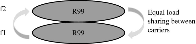
Figure 11.6 Load sharing between Release 99 carriers
Typically the second carrier deployment at this stage was not done for large contiguous areas but rather only for hotspots and, therefore, the second carrier cell coverage was much larger than that of the first carrier. This is due to the lower interference levels on the second carrier, which do not have direct adjacent cell neighbors like the first carrier cells have. In this scenario, all UEs must be directed to the first (contiguous) carrier very aggressively in idle mode. To achieve this, a negative Qoffset2 is used for first carrier neighbors on the second carrier, as shown in Figure 11.7.

Figure 11.7 Pushing UEs to f1 in idle and dedicated mode
Similarly, in dedicated mode the UEs must be pushed to the first carrier and the inter-frequency handover has to be triggered based on RSCP threshold rather than Ec/No. The reason for this is that good Ec/No areas in the second carrier can extend over several first carrier neighboring cells and can over complicate the neighbor planning. Therefore the inter-frequency handover should be triggered on RSCP instead (typical values of around −103 dBm are recommended, although this greatly depends on the specific sector situation). Each second carrier cell should be configured with inter-frequency neighbors from the first carrier of the same sector, in addition to inter-frequency neighbors extracted from the intra-frequency neighbor list of the first carrier.
11.3.1.2 Early Layering for HSDPA
At the initial phases of HSDPA deployment, the layering strategy can be very simple, just add HSDPA on the second carrier and keep all Release 99 on the first carrier as shown in Figure 11.8. This way the additional interference caused by HSDPA activation does not affect voice traffic (note that HSDPA typically uses full base station power during the transmission).
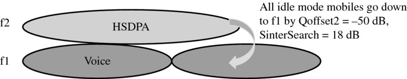
Figure 11.8 Early layering strategy with HSDPA
The neighboring strategy can follow the same as that described in the Release 99 layering scenario. This type of layering strategy causes some challenges:
- In order to have all the voice calls on the first carrier the UEs should be moved to the first carrier immediately after the release of HSDPA (or Release 99 packet call) call on the second carrier. This causes extra signaling load on the first carrier due to cell updates in the case that the UE was in cell_PCH state.
- As each call is always initiated on the first carrier, the signaling load on the first carrier could cause extremely high load. The signaling traffic can lead to higher uplink noise rise due to heavy RACH usage, which can impact the coverage area of the first carrier.
- As HSDPA is only served on one single carrier, the throughput per user can degrade rapidly as the HSDPA traffic increases. In case of non-contiguous HSDPA layer, the HSDPA service would only be available in certain hotspots.
Figure 11.9 shows that most connection establishments are HSDPA packet calls. This is explained by the fact that smartphones can create very frequent data connections compared to the number of voice calls. Therefore, using the initial layering setup would lead to several carrier changes for roughly 98% of the calls. This would mean excessive signaling load with increased uplink noise rise on the first carrier.
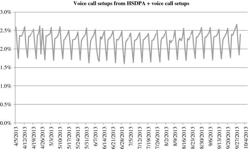
Figure 11.9 Share of voice call connection establishments
As the HSPA service grows, the layering strategy should be adjusted as described in the following section.
11.3.1.3 Layering with Increasing HSDPA Traffic
The rapid HSDPA traffic increase, decrease of HSDPA throughput per user and the signaling traffic explosion due to the continuous layer changes, required a modification of the layering strategy, as shown in Figure 11.10.
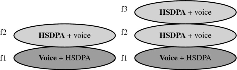
Figure 11.10 Layering with increased HSDPA traffic
This layering strategy means the UEs are no longer pushed to the first carrier but rather voice or HSDPA calls are handled by the layer the UE happens to select, or is directed to due to load balancing.
There are two main traffic balancing strategies:
- a symmetric layering strategy, in which both voice and data are balanced in all layers (symmetric layering strategy), or an
- asymmetric layering strategy, in which voice tends to be mainly in one layer that has little data traffic (asymmetric layering strategy).
In this second case, the load balancing can be done based on the number of HSDPA users so that carrier 2 (and 3 or 4) handle most of the HSDPA calls while carrier 1 handles most of the voice calls. In networks with this configuration, typically 70–80% of all HSDPA calls are equally shared among HSDPA carriers 2 and 3, while 70–80% of voice calls are allocated to carrier 1.
At the border of any carrier the neighbors need to be set according to Section 11.3.1.1 that is, all UEs at the coverage border of certain carrier should be directed to any of the continuous coverage carriers. Further load balancing at the coverage border of certain carrier can be done so that idle mode cell reselection is targeted to a different carrier than dedicated mode handover, as shown in Figure 11.11.
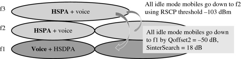
Figure 11.11 Handling of UEs at the carrier coverage border
11.3.1.4 Layering with HSUPA
When HSUPA was activated, the layering strategy was typically such that HSUPA was activated together with HSDPA. This caused a rapid increase of uplink noise rise as indicated in Figure 11.12 which shows the Received Total Wideband Power (RTWP) in an example network over a period of three months. This network used an asymmetric balancing layering strategy (i.e., voice preferred in carrier 1).
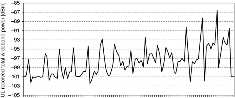
Figure 11.12 HUSPA (E-DCH) selections increase of RTWP
The RTWP increased from −101 dBm to −93 dBm (8 dB noise rise) in about three months, and the E-DCH channel selections increased by a factor of 5. The cell range was reduced due to the higher noise, which caused an increase in the dropped call rate for voice.
This increase in dropped call rate can be optimized by changing the layering strategy so that HSUPA is activated only on non-voice prioritized layers, as shown in Figure 11.13.
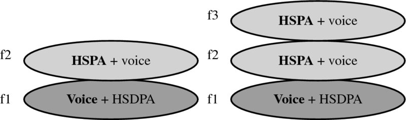
Figure 11.13 HUSPA activation on non-voice prioritized layers
For each carrier the impact of HSUPA activation on uplink noise rise must be well controlled in order to maintain the same coverage footprint. In addition to the deactivation of HSUPA, which is a rather extreme measure, Chapter 12 describes other techniques that can help mitigate the increased noise rise caused by smartphone traffic.
With the introduction of dual-cell HSDPA (DC-HSDPA) at least two carriers should be used everywhere in the network where DC-HSDPA capability was required. In cases with three carrier contiguous deployments, the DC-HSDPA can be activated in the second and third carrier leaving the first carrier slightly less loaded and therefore offering a better quality (Ec/No). This higher quality can be utilized when terminals are making handovers or cell resections from GSM and also as a fall-back layer within the WCDMA network (used before handing over to GSM). In the case of four carrier deployment in WCDMA, two DC-HSDPA cell pairs can be configured, that is, one for carriers 1 and 2 and another one for carriers 3 and 4. It should be noted that the primary cell of DC-HSDPA must (typically) have HSUPA activated and therefore the carrier that has the largest HSUPA coverage should be selected as the primary cell.
11.3.1.5 Layering with GSM
The GSM layer is used as a fall-back layer where the UEs are directed in idle and connected mode due to lack of coverage. The idle mode threshold for Ec/No is typically around −16 dB Ec/No with minimum rx level at around −101 dBm as shown in Figure 11.14. In this particular example, the GSM layer is in the 900 MHz band and UMTS in the 2100 MHz band.
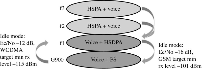
Figure 11.14 Layering between G900 and U2100
Handover to G900 is initiated at around −110 dBm RSCP level and/or at around −16 dB Ec/No. Handovers and idle mode cell reselection to G900 is only triggered from the first carrier and therefore G900 neighbors are only defined between G900 and U2100 first carrier. Return from G900 to U2100 first carrier (or alternatively also to second carrier if that is continuous) should not happen in idle mode until −12 dB Ec/No in U2100. Typically handovers from G900 to UMTS for voice are only defined based on G900 load, for example, at 80% time slot utilization in GSM triggers the handover to U2100 provided that Ec/No target of −12 dBm and RSCP of −115 dBm are fulfilled. Figure 11.14 illustrates the traffic movement across layers.
11.3.2 Layering Strategy with Multiple UMTS Bands
Layering strategy with multiple WCDMA bands greatly depends on the number of carriers on different frequency bands. The most typical deployment scenario is that the low band (at 900 MHz i.e., U900 or at 850 MHz i.e., U850) has fewer carriers than the high band U2100. This means that in order not to overload the low band carrier(s) the UEs must be pushed aggressively to U2100 and the fewer low band carriers there are, the more aggressively UEs need to be pushed to the high band. Otherwise the low band cell will be highly loaded (practically blocked) due RRC connection requests or cell update signaling. Figure 11.15 shows the typical case which is used as an example scenario in the detailed analysis throughout this chapter.
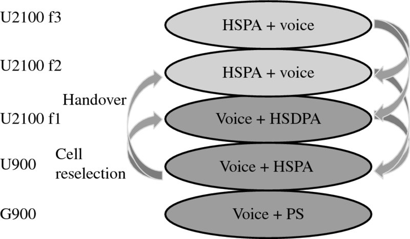
Figure 11.15 Typical multiband layering scenario for WCDMA
The multiband layering scenario in Figure 11.15 shows that there are no handovers or cell reselections to the G900 layer any more, except at the U900 coverage border where idle and dedicated mode mobility between WCDMA and GSM can be as shown in Section 11.3.1.5. The traffic sharing between U900 and U2100 layers can be done so that in idle mode all the UEs are pushed aggressively from U900 to the first carrier of U2100 and handovers from U900 are towards the second U2100 carrier to balance the load, provided that the second U2100 carrier has continuous coverage.
11.3.2.1 Multiband Layering Parameters
In this section some of the most critical design aspects of layering between U2100 and U900 are discussed in detail.
Idle Mode
Figure 11.16 shows the importance of Sintersearch parameter setting at the U2100 layer. In the case that the Sintersearch is set too high and therefore UEs start to measure U900 very early (at high Ec/No values at U2100 layer) and reselect aggressively to U900, the RRC setup success rate and RRC success rate (1-RRC drop rate) collapses. The worst values for RRC setup success rate are around 10%, indicating that the single U900 carrier cannot handle the traffic from three or four U2100 layers. Therefore the UEs should not be allowed to even measure the U900 carrier until the quality (Ec/No) at the U2100 layer falls to around 6 dB above the minimum acceptable Ec/No limit. This, combined with the Qoffset for RSCP of around 4 dB and Ec/No around 2 dB (both requirements mean U900 should be better than U2100), can protect the U900 layer from getting too much traffic from U2100.
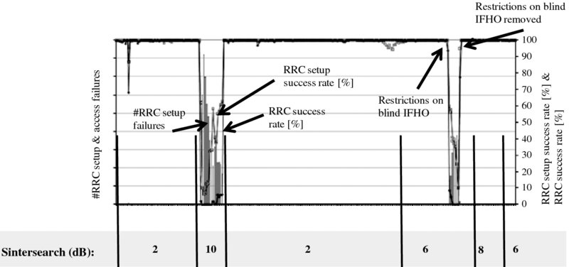
Figure 11.16 Importance of SinterSearch
The reselection from U900 to U2100 should be very aggressive, basically measuring all neighbors (intra- and inter-frequency) all the time and having 2–4 dB negative offsets for RSCP and Ec/No thresholds at the U2100 layer. The negative offset means that U2100 quality can be lower than U900 for the reselection. The reselection from U900 to the first carrier of U2100 should be performed quite early, as the first carrier of U2100 has less HSDPA (and no HSUPA) traffic and therefore Ec/No performance is better than for other U2100 carriers.
Dedicated Mode
In dedicated mode, the handover target (U2100) carrier should be different from the idle mode reselection target carrier. The idle mode target is the first frequency while the handover target could be the second frequency, provided that there is more than one single continuous coverage layer in U2100. Then, similarly to the idle mode control, the UEs must be pushed to the second U2100 carrier as soon as possible. This can be done by using, for example, blind handover during the RAB setup phase where the handover from U900 to U2100 is triggered without any inter-frequency measurements. This blind handover can be also assisted by intra-frequency measurements from event 1a or 1c, or any periodic RSCP reporting that might active, or then by inter-frequency RSCP measurement report from RRC connection request and/or cell update messages. Based on these measurement results the handover is not entirely blind as some information about target cell RSCP is available. Then, the handover from U900 to U2100 can be triggered based on either real U2100 target cell RSCP or U900 source cell RSCP offset by a threshold to take the penetration loss difference between the bands. The blind handover (or blind handover assisted by measurements) performance is very sensitive to the antenna directions for different bands. If there is even a slight difference between the antenna directions of the two band cells, the blind handover performance suffers greatly unless the target cell (U2100) RSCP measurements are not available from RRC connection request or cell update messages. Figure 11.17 shows the blind handover success rate for a sector where U900 and U2100 have individual antennas around 6 degrees difference in directions. The blind handover success rate cannot reach >90% levels even if the threshold for own cell (U900) RSCP is increased from −95 dBm to −90 dBm. It should also be noted that when RSCP threshold is increased the traffic in the U900 layer increases, causing excessive load in the U900 layer. It should be noted that failure in blind handover does not cause any dropped call or setup failure from an end user point of view. If the blind handover fails, the UE returns to the old (U900) carrier.
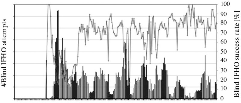
Figure 11.17 Blind handover success rate
Another possibility is to use compressed mode and actual inter-frequency measurement at the end of the packet call. This is done so that, instead of moving the UEs to Cell_PCH, URA_PCH, or idle mode, the UEs are ordered first to compressed mode and in the case that the U2100 carrier is found to have adequate RSCP and Ec/No the handover is executed instead of moving UE to cell_PCH, URA_PCH, or idle mode. This way the achievable handover success is around 98 – 99%.
Handovers from U2100 to U900 should only be done in the case of lack of coverage in the U2100 layer. And in the case of hotspot coverage for certain U2100 carriers, the handover should be first done to the continuous coverage carrier within the U2100 layer before handover to the U900 layer. The handover thresholds from U2100 to U900 are typically set to be similar to the previous chapter's U2100 to G900 handover thresholds, as discussed in Section 11.3.1.5.
11.3.2.2 Neighbor Planning
The neighbor relations are planned so that from each U2100 carrier having continuous coverage there are neighbors to the U900 carrier of the same sector (same BTS) and inter-BTS neighbors are only needed in the case that the antenna directions between the same sector bands are not the same. Intra-band neighbors within the U2100 carriers of the same sector are not defined except in the case of U2100 channel border areas. This can be done provided that the traffic between the U2100 carriers is equally distributed. G900 neighbors are also only defined in the case of U900 border.
11.3.3 Summary
The layering between different WCDMA carriers within the same band or different bands should try to balance the load between all the carriers. Load here can mean number of HSPA users, voice erlangs, and signaling. It is especially important to monitor the signaling traffic (number of RRC connection requests and cell updates) which can increase rapidly and block one of the carriers. Therefore, equal sharing of UEs among all carriers is mandatory. This means that some parameter tuning needs to be performed from time to time as the total traffic increases.
11.4 RAN Capacity Planning
Capacity planning and system dimensioning is an important aspect when operating a wireless communication service. A balance must be struck between over-dimensioning the system, leading to premature capital expenditures, and under-dimensioning the services provided, which can lead to poor customer experience and even customer churn. Historically, statistical models such as the Erlang B model have been used by wireless operators to estimate the voice service GoS (Grade of Service) they are providing to their customers. Once it is forecasted that the BH (Busy Hour) erlangs of a cell may result in a blocking rate of 1–2%, additional voice trunks or circuits are provisioned to improve the GoS below the targeted threshold. Dimensioning the data services is much more challenging due to their more bursty nature compared to voice and the fact that many different services can run over data channels that have vastly different service requirements. For example, data services such as email or MMS have a much more relaxed delivery delay requirement compared to real time services such as video or music streaming. Unfortunately, RAN (Radio Access Network) KPIs really don't tell the whole story because the counters blend many data services with different service requirements together. As discussed in Chapter 13, the real customer experience should be estimated with new KPIs that measure the performance of each service independently. Since those application specific KPIs are not available yet, this section reviews some of the RAN (Radio Access Network) KPIs that might give us some insight into the average customer experience.
11.4.1 Discussion on Capacity Triggers
For HSPA+ data services, the customer demand can be measured in terms of MB volume transferred over the air interface. The average sector throughput of a cell is an important metric because it shows the potential amount of data that can be transferred during an hour and the throughput speed gives an indication of what services on average can be supported. The average throughput a sector can support is a function of the user geographical distribution inside the cell footprint. In general, if most of the users are near the NodeB, the cells' throughput is higher than in a cell where most of the users are in poorer RF condition on the cell edge. One metric to monitor closely is the cell TTI (Time Transmission Interval) utilization. In HSPA, the length of one TTI is 2 ms, hence there are theoretically 1.8 million TTIs that can have customer payload per hour. Once all the TTIs are utilized the cell is sending the maximum MB volume that it can support. Figure 11.18 (left) plots the DL MB volume vs. the TTI utilization. For this particular cell, the maximum MB customer demand it can support during the busy hour is approximately 700 MB. The slope of the line in the graph is the weighted average HSDPA throughput of 1.7 Mbps.
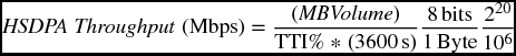
Figure 11.18 HSPA+ cell capacity and loading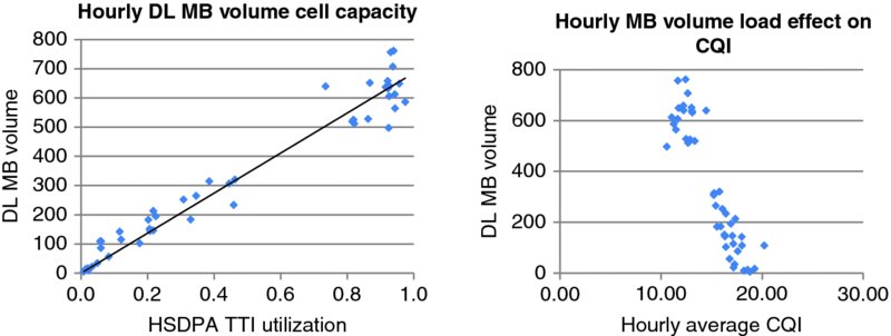
Figure 11.18 (right) shows the effect on the CQI (Channel Quality Index) beginning reported by the mobiles' as more data is sent over the HSPA+ air interface and the system loads up.
The TTI utilization is an indication that a cell is at its maximum capacity; however, what we really need to know in order to dimension the system is what the average user experience is when the cell is loaded. Since the HSDPA air interface is a shared resource in the time domain it is important to try to measure the throughput a typical user will see as other users are added to the system. Measuring the delay of the entire system is the goal for data networks, so queuing models such as Erlang C may be utilized. There is one scheduler assigned per cell on an HSPA+ NodeB, so essentially there is a single server and we can look at the TTI utilization in terms of erlangs of scheduler utilization and model the total system delay as an M/M/1 queue [5] which is a specific case of Erlang C where the number of servers or channels is equal to one. Figure 11.19 illustrates the concept. For data traffic, we are interested in the queuing delay because it will give us an indication of the entire systems' performance as perceived by the customer. For an M/M/1 queue the average total system delay (TA) can be expressed as:
Figure 11.19 Generic queuing model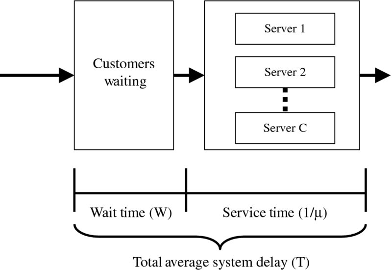
Where WA is the wait time (queue time), 1/μ is the average service time, and p is the server utilization (TTI%). For an HSPA+ system, WA is the average time customer data is waiting to be scheduled at the scheduler, the service time is the average time it takes to send the customer data over the air interface. The service time is a function of the total time it takes to deliver data and the TTI utilization. The customer's perception of time will be the total time TA, while the networks' perception of time is 1/μ.
The same customer data that is sitting in the scheduling queue is also sent over the HSDPA air interface, so we can express the above time domain expression in terms of throughput.
Where RU is the average end user's perceived throughput and RS is the average sector throughput. A good rule of thumb is that at 90% TTI utilization the user experience is only 10% of the sector throughput, at which point the poor data throughput is probably very noticeable to the customer. Another important insight to the M/M/1 model is that as the TTI utilization approaches 100%, caused by a large amount of users in the system, the user perceived average throughput approaches zero, which implies that there is an infinitely long queue of data waiting to be scheduled.
Figure 11.20 shows the hourly statistics collected over a two-day period for a single highly loaded cell. When the TTI utilization approaches 100% the sector throughput still looks fine, but the user experience from 9:00 to 17:00 is below an acceptable level. Also, the user perceived throughput calculated via the M/M/1 queue model closely matches the HSDPA average user throughput as reported by the RAN counters, which are measuring the amount of data in the scheduler buffer. The degraded CQI that is reported by the mobiles as the system becomes loaded and the high TTI% utilization have a compounding effect on the customer experience. The former reduces the potential throughputs that a mobile can get when it is scheduled and the latter is an indication of how often it has to wait before it can be scheduled.
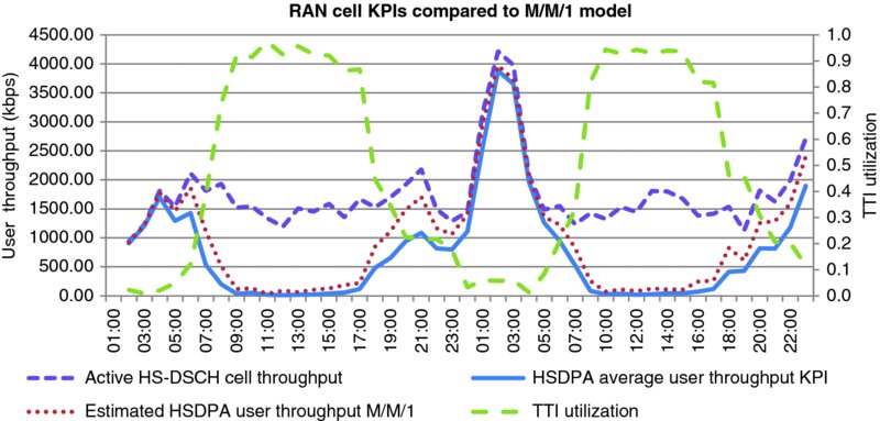
Figure 11.20 Cell and user throughput KPIs in a loaded sector
11.4.2 Effect of Voice/Data Load
UMTS supports both CS R99 voice and HSPA+ PS data services on the same carrier. The NodeB transmit power is a key air interface resource that is shared between voice and data services. To support the pilot and common control channels, 15–25% of the cell PA (Power Amplifier) is utilized. Downlink power is a shared resource, therefore the voice traffic has big impact on the available power that can be used for HSDPA data services. Often the voice channels consume more than half of the PA power, even though the data services represent the larger portion of the cell capacity.
The following example is extracted from a network with a significant voice traffic load. On the loaded cell shown in Figure 11.21 over 60% of the power is used to support R99 voice during the busy hour. The remaining 40% of the average power of the PA can be used during peak times to support HSDPA. However, from a spectral efficiency perspective the HSDPA payload represents nearly 80% of the cell capacity, while the voice represents only 20%.
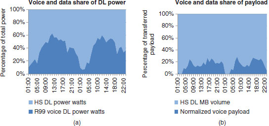
Figure 11.21 Comparison of voice and data power (a) and data (b) consumption in a loaded sector
The RAN KPIs only report the average HSDPA power over an hour. However, if very few TTI are used during the hour the average HSDPA traffic will be very low, even though when it was in use the power may have consumed all the remaining PA power that was not being used for R99 voice. For the same cell that was analyzed above, Figure 11.22 shows the average hourly HSDPA power vs. the TTI utilization over the same two-day period. Note that no more average power can realistically be allocated to HSPA+ because nearly all the TTIs are in use during the busy hour. For the same cell, not unsurprisingly the DL HSDPA power is also highly correlated to the MB volume of HSDPA data.
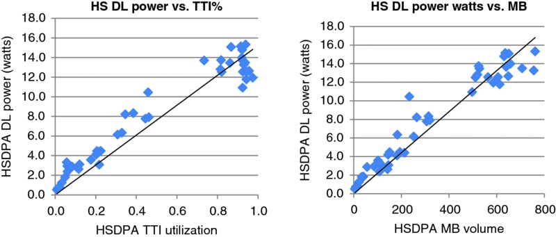
Figure 11.22 Impact of TTI utilization and data payload on HSDPA power consumption
In smartphone dominated markets the majority of the capacity on a UMTS cell is represented by the HSPA+ data, even though it may appear that most of the power is being utilized for R99 voice.
11.4.3 Uplink Noise Discussion
The uplink capacity is also a very important consideration when evaluating capacity solutions. In terms of spectral efficiency, HSDPA Release 8 is 3–4 times more spectrally efficient than Release 6 HSUPA, so theoretically the uplink should not be a bottleneck until the ratio of downlink traffic payload to uplink traffic payload is on the order of 4 : 1. In a smartphone dominated network, the ratio of downlink to uplink traffic volume is on the order of 7 : 1 or even greater because much of the data transferred in the network comes from downlink dominated applications such as video streaming. However, in live networks 30–60% of congested sites experience uplink capacity issues, which isn't consistent with the spectral efficiency expectations. There are also significant differences across infrastructure vendors, with some vendors being more prone to uplink congestion, as illustrated in Figure 11.23.
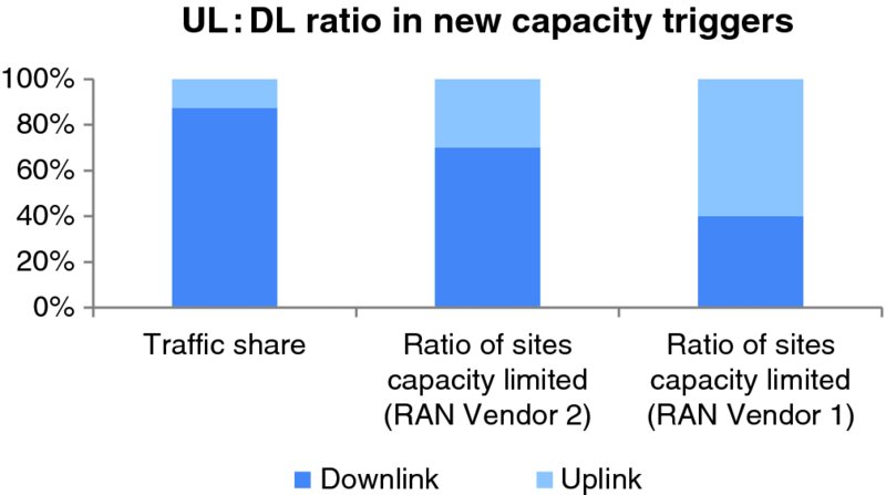
Figure 11.23 Comparison of DL/UL traffic share vs. capacity triggers
Due to the bursty nature of the smartphone traffic, the uplink direction will experience a large number of bearer allocations, releases, and very short data sessions. As Figure 11.24 illustrates, the power in the uplink is dominated by HSUPA, even though it is not necessarily the main source of payload. Chapter 12 will provide a deep analysis of the reasons for the excessive uplink noise that is observed in networks with heavy smartphone traffic, and possible optimization actions to mitigate this problem.
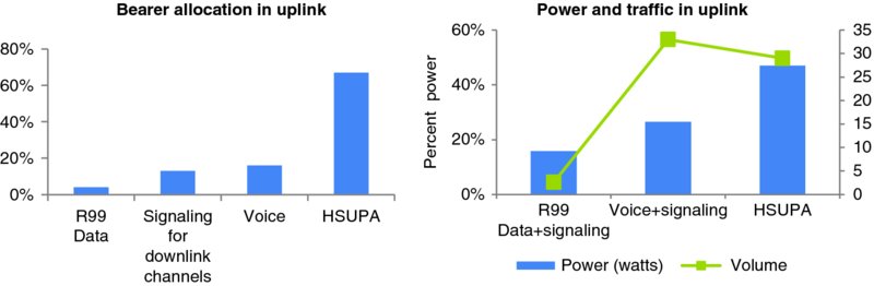
Figure 11.24 Power and payload breakdown in uplink based on service and channel type
As the noise rises in the NodeB, the devices must increase their transmit power to hit the required BLER targets, which in turn generates more uplink noise. There comes a point where the mobile device is at full power but the signal received by the NodeB is too low to be detected, which can lead to access failures and poor uplink performance in terms of throughput.
The goal of determining the uplink capacity for a sector is to estimate the point at which the uplink noise rise becomes so high that uplink throughput is impacted and other real time services, such as voice, begin to experience congestion. When HSUPA 2-ms TTI is deployed it is possible that the uplink noise rise of the system may approach 8–10 dB in heavily loaded cells. When this much noise rise is experienced, system KPIs – such as access failures – begin to degrade. As the noise rise increases, typically data traffic is affected first, followed by voice traffic and eventually SMS services.
In cells with high uplink congestion the number of active users is nicely correlated to the number of data sessions. Three cells with high noise rise in three different areas of the same network were analyzed. There is a ratio of 300–400 data sessions per active user. In Figure 11.25, hourly RAN KPI data is plotted to show the relationship between active users and the uplink noise rise throughout a couple of days. As the average number of active users is trended into the 20–30 range, the uplink noise approaches the 8–10 dB uplink noise threshold.
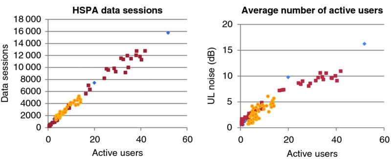
Figure 11.25 Impact of number of simultaneous users on UL noise rise
During events where there is a high concentration of smartphone devices in a small geographical area, such as a sports stadium or convention center, the noise rise can quickly escalate to over 10 dB, after which point the network KPIs and customer experience are dramatically affected. Figure 11.26 shows a cell that serves a sports stadium with thousands of spectators. The chatty traffic generated by the smartphone helps increase the uplink noise, leading to very high levels of system access failures.
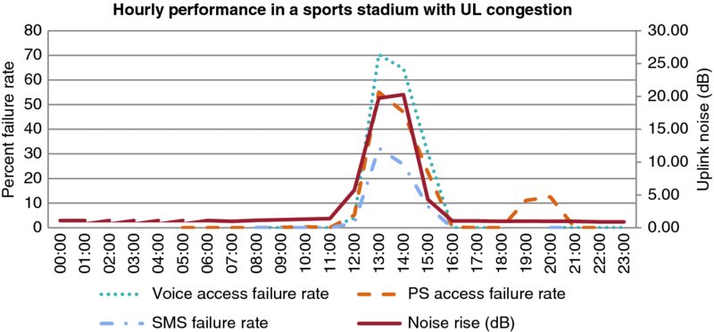
Figure 11.26 Extreme UL noise during mass events
Stadiums that serve major sporting events can have a user demand that is nearly 20 times that of an average cell site. They are very challenging from a system capacity planning perspective because the high concentration of smartphones lasts only a few hours, during only a few days a month. A very high capacity system must be deployed to augment system capacity so that the customer experience can be maintained. Typically, neutral host DAS (Distributed Antenna Systems) are deployed with the support of the stadium owners to help operators support the high density of customer demand. In high density device scenarios it is critical to deploy enough geographically separated cells such that they split the uplink traffic so that the full capacity of the downlink can be utilized.
11.4.4 Sector Dimensioning
Capacity planning limits were discussed earlier in Section 11.4.1. These capacity triggers assumed that the RF air interface was the capacity bottleneck. Once these capacity triggers are reached additional sector capacity is needed to meet the growing data demand. As a pre-requisite to measuring the capacity triggers on the RF air interface, the site baseband capacity and IP Iub capacity limits need to also be checked to make sure they are not limiting the RF capacity. These capacity constraints are discussed in the next section and Section 11.5 respectively.
Once it has been verified that the RF capacity is the bottleneck and capacity triggers such as high TTI utilization are measured, as discussed in Section 11.4.1, the next step is to determine if the congested sector throughput is also good. If the sector throughput is good, the quickest and most cost effective solution is to add an additional carrier frequency. If there are spare baseband and power amplifier resources available the activation of a carrier can even be performed without a site visit. In order to mitigate the performance impacts of handling multiple carriers, as discussed in Section 11.3, it is often good practice to add carriers not only to the site that needs it but also to some of the neighboring sites that have high interaction rates with the congested sector.
Congested sectors with poor throughput will also benefit from additional carriers, however carrier adds are not a long-term solution to providing additional network capacity. For these sectors, more investigation is needed to help determine why the sector throughput is sub-standard. Sector optimization techniques, as discussed in Section 11.2.2, may be needed to improve the SINR in the coverage areas that are generating the traffic demand. If it is determined that the traffic is being generated in poor coverage areas that can't be improved by optimization, or that a sector is already utilizing all the carrier frequencies that are available to the operator, the next option is to build additional macro sites or micro sites to improve the coverage in the poor RF areas and expand the overall network capacity.
11.4.4.1 Optimization of RAN Baseband Resources
When data traffic increases in the network, the throughput offered to the existing users will be reduced. When the throughput levels reach certain quality limits determined by the operator, the capacity of the network will have to be increased.
While this is expected from any technology, and typically fixed adding more data channels (UMTS carriers), in the case of HSPA+ there is an intermediate step that needs to be considered: incrementing the baseband capacity of the site.
In heavily loaded sites, the lack of baseband resources can play a major role in performance. The effect is the same as normal radio congestion – throughput reduction – however in the case of baseband shortage the scheduling rates are typically low. This can be seen during drive tests, which will show a high DTX rate in the transmissions, or in the network KPIs, with a low TTI utilization or lack of HS-PDSCH codes.
Consider the example in Figure 11.27, in which one cluster was presenting low overall throughputs (2.2 Mbps per carrier) even though the radio conditions were decent. It was found that three sites in the cluster required an upgrade on their baseband resources, which resulted in 100% improvement of the throughput in the cluster, to an average of 4.4 Mbps.

Figure 11.27 Throughput improvement after baseband upgrade. Low baseband case (left) presents a high number of low throughput dots (dark gray)
One important thing to consider is that baseband shortage can occur even in cases with relatively low amounts of transferred data, especially in networks with a high penetration of smartphone devices. In the example above, even during the night time there were at least 19 HSPA customers connected to the site. The HSPA users in connected mode will consume baseband resources even if they are not actively transmitting data; as will be discussed in Chapter 12, it is possible to adjust the state transition settings to limit this impact, at the expense of longer connection latency.
11.4.5 RNC Dimensioning
The RNC (Radio Node Controller) serves as an anchor for mobility management and radio resource management in an HSPA+ network. The dimensioning of the RNC is important because it will degrade the performance of multiple NodeBs for reasons not related to the air interface capacity, so it can often be difficult to troubleshoot. Below are some common parameters used to dimension the RNC:
- Aggregate Throughput (Mbps);
- Number of NodeBs and Cells;
- Number of Active Users;
- Processing Load.
Originally, RNCs were designed to focus on throughput capacity as their main bottleneck; however, in smartphone dominated networks it became clear that the signaling capacity could rapidly become a bottleneck as well. Figure 11.28 shows that there are situations in which the signaling capacity (Y axis) can be exhausted well before the RNC has been able to achieve the designed throughput capacity (X axis).
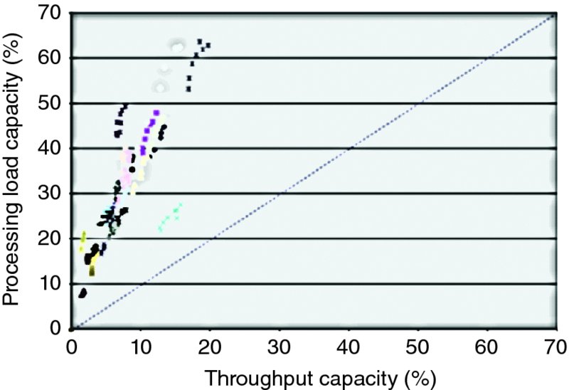
Figure 11.28 Illustration of RNC capacity bottlenecks: Y axis shows control plane capacity, X axis shows user plane
As RNCs are added to the network to keep up with increasing smartphone penetration, sites need to be “re-homed” from their original RNC; this leads to more RNC handovers, and an additional operational complexity derived when a large number of NodeBs need to be logically “re-built” and configured on new RNCs.
There are important differences in vendor RNC design, with some vendors providing a more flexible architecture that enables the “pooling” of resources for either the control or user plane, thus facilitating the balance of the processing capacity and delaying the need to increase the number of RNCs as traffic increases.
11.5 Packet Core and Transport Planning
While not as complex to plan and tune as the radio network, it is important to properly plan the core and transport networks to ensure they provide the required bandwidth and latency for the data services being offered. In this section we discuss some considerations regarding the planning of the Serving GPRS Support Node (SGSN) and the Gateway GPRS Support Node (GGSN).
Modern HSPA+ networks typically implement the GTP one tunnel solution, which tunnels the user data transfer directly to the GGSN, effectively leaving the SGSN to primarily handle data signaling traffic. GGSNs, on the other hand, will be the main node dealing with user data transfer and are specialized to cope with large amounts of data volumes.
When dimensioning the packet core, the number of SGSNs will be related to the amount of sessions being generated, while the number of GGSNs will depend mostly on payload and number of PDP contexts that can be sustained.
SGSN configuration and dimensioning will also be impacted by the PS paging load in the network. If the paging load is too high, the routing areas will need to be made smaller.
SGSNs can be configured to distribute the data sessions in one area across multiple GGSNs. This is known as “pooling” and can be used as a way to avoid over-dimensioning; however, it may have negative effects on user experience as it will be discussed later on this section.
In addition to SGSN and GGSN, many networks deploy a wireless proxy, whose goal is to improve data performance and reduce network payload. There are many flavors of proxies, however they typically implement the following features:
- TCP Optimization, which provides advanced methods to compensate for typical TCP problems in wireless environments.
- Image and text optimization, which reduces image and text payload by compressing or resizing images.
- Video optimization, targeted at reducing video payload while providing an optimum user experience.
While network proxies can help reduce overall payload, their effectiveness will decline as more traffic is encrypted, which limits the possible actions the proxy can take.
As discussed earlier, another important consideration regarding core network dimensioning is latency. Packet delay is a major factor affecting data user experience: HSPA+ networks will not be able to perform at the highest level if there are long delays. This is due to side effects from the TCP protocol, which mistakenly interprets long delays as if data was being lost in the link.
One of the most important considerations to optimize latency in the network is the placement of the GGSNs. In networks covering wide territories it is recommended to distribute the GGSNs to try and have them as close as possible to where the traffic originates. Figure 11.29 shows an example network in which the overall round-trip delay was reduced by an average 22 ms when the GGSNs were distributed, as compared to a centralized deployment.
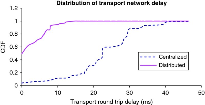
Figure 11.29 Example transport network delay in a centralized vs. distributed deployment
11.5.1 Backhaul Dimensioning
As the RAN (Radio Access Network) has evolved from sub 1 Mbps to multiple Mbps speeds it has become clear that legacy T1 (1.544 Mbps) or E1 (2.048 Mbps) speeds that were used to support circuit switched voice would no longer be able to scale and support the data speeds that would be achievable on HSPA(+) and LTE networks. Ethernet backhaul became an attractive replacement based on its common availability, ubiquity in the Internet industry and support of speeds that could scale proportionally at a reasonable cost for the expected increase in data demand. Common Ethernet rates scale from 10 Mbps Ethernet (10BASE-T), to 100 Mbps Fast Ethernet (100BASE-TX) and even 1 Gbps Gigabit Ethernet speeds and beyond.
High speed wireless data networks often advertise peak data rates. These peak rates are the maximum a technology can provide and can realistically only be measured in a lab environment under near perfect RF (Radio Frequency) conditions. It is important when dimensioning the Ethernet backhaul that we look at how these RAN (Radio Access Network) technologies are deployed and what other constraints limit the available speeds that a customer may realistically be able to achieve in a real wireless network if there were no backhaul limitations. Peak data rates provide a ceiling for what is achievable from a wireless technology, but they are almost never realized in a real operating environment. The support of high peak data rates is important from a user experience point of view, since data is sent in bursts; however the application requirements for these bursts are not so high. As referenced in Chapter 13, peak bursts of 11 Mbps were observed when streaming a Netflix movie.
Average spectral efficiency is often used to estimate the capacity a wireless network can provide. However, using average throughput to dimension backhaul may underestimate the amount of time that the customers' throughput is limited by the provisioned Ethernet backhaul bandwidth. The following approach attempts to adjust the peak throughput ceiling to more realistic throughput targets. HSPA+ utilizes higher order modulation, such as 64QAM modulation, to achieve the peak data speeds which requires very good SNR (Signal to Noise). However, network statistics show that the RF environment is good enough to utilize 64QAM modulation typically less than 20% of the time. Also, under more realistic network conditions, more FEC (Forward Error Correction) is needed when the SNR decreases, so the achievable speeds are further reduced.
Table 11.5 shows some target throughputs based on the following assumptions:
- Reduce the peak throughput by a factor of 1.5 (difference between 6 bits/symbol 64QAM and 4 bits/symbol 16QAM).
- More realistic throughput using an effective coding rate of 6/10, which is based on the maximum throughput of 16QAM in the 3GPP CQI tables.
- Using these two correction factors we see the target throughputs scale down to approximately 40% of the peak speeds the RAN can theoretically support.
Table 11.5 –Realistic peak HSPA+ speeds for Ethernet backhaul dimensioning
| Technology/downlink spectrum | Downlink theoretical peak (Mbps) | Theoretical without 64QAM modulation (Mbps) | Realistic peaka without 64QAM modulation (Mbps) |
| HSPA+ 21 (5 MHz) | 21 | 14 | 8 |
| HSPA+ 42 (10 MHz) | 42 | 28 | 17 |
aNote: Realistic peak speeds assume an effective coding rate of 6/10, which is based on 3GPP CQI mapping tables for 16QAM modulation.
Backhaul is a shared resource between sectors of the same site, so there are trunking efficiency gains that can be realized when HSPA+ is initially deployed and it is assumed that only one sector will be in use during a given TTI (Time Transmission Interval). Table 11.6 shows some example backhaul dimensioning calculations. If we had used the theoretical peak speeds to dimension the system we would need approximately 125 Mbps of backhaul to support a site that had HSPA+ 42 (dual carrier) on all three sectors. Based on the example calculations, for the initial deployment of these high speed technologies they can realistically be supported by as little as 1/7th of the maximum air interface speed summed across a three sectored site. This assumes only one sector per site will be busy initially, but as the traffic grows multiple sectors may be utilized at the same time, so the backhaul will need to be augmented accordingly to maintain an adequate Grade of Service (GoS) to the customers. However, care must be taken to also check that applications that customers are using are actually requesting the peak speeds that the air interface is capable of supporting. Incremental capacity should also be added to support the control plane usage, but it is expected that this only adds as much as an additional 4–6% to the overall backhaul requirement.
Table 11.6 Recommended backhaul dimensioning by technology
| Technology/downlink spectrum | Ethernet backhaul typical traffic (Mbps) | Ethernet backhaul heavy traffic (Mbps) |
| HSPA+ 21 (5 MHz) | 20 | 20 |
| HSPA+ 42 (10 MHz) | 20 | 50 |
| 3–4 HSPA+ carriers | 50 | 100 |
11.6 Spectrum Refarming
11.6.1 Introduction
The concept of refarming is borrowed from agriculture, where many scattered plots of land are consolidated and redistributed among the owners. In wireless, refarming refers to the consolidation of spectrum assets in preparation to their use for the new radio technology. The typical case is to deploy HSPA or LTE technology on the existing GSM frequencies at 850/900 MHz and 1800/1900 MHz. The motivation for refarming is to get more spectrum for growing HSPA traffic and to improve the HSPA coverage by using lower spectrum with better signal propagation. The North American and Latin American networks use 850 and 1900 MHz refarming for HSPA, most European operators and some African operators have deployed HSPA on 900 MHz band, and both 850 and 900 MHz frequencies are used for HSPA in Asia. Some of the 900 MHz networks are also new spectrum allocations, like the world's largest UMTS900 network run by Softbank in Japan. The GSM 1800 MHz spectrum is also being refarmed to enable LTE deployments.
Refarming UMTS to the low bands 850 and 900 MHz provides a major benefit in coverage. The typical coverage area of a three-sector base station in an urban area is shown in Figure 11.30. The coverage calculation assumes the Okumura-Hata propagation model, a correction factor of 0 dB, a base station antenna height of 25 m, indoor loss of 15 dB, slow fading 8.0 dB, and required location probability of 95%. The antenna gain at low bands is assumed to be 3 dB lower than at high bands. The coverage area of 900 MHz is nearly 3 times larger than at 2100 MHz. The difference between 850 and 1900 MHz coverage is also similar. The better coverage is a major motivation for the operators to deploy UMTS on the low spectrum. The coverage improvement helps not only for the rollout in rural areas but also improves the indoor coverage in the urban areas.
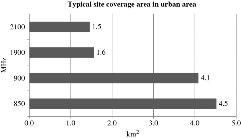
Figure 11.30 Coverage area of 3-sector cell site in urban area with 25 m base station antenna height and 15 dB indoor penetration loss
Another motivation for the GSM band refarming is the wide support of multiple frequency bands in the devices: in practice all new 3G devices support UMTS900, or UMTS850, or both bands, and also most devices already out in the field support the low bands. Therefore the deployment of UMTS900 or UMTS850 can provide coverage benefits for the existing devices too.
11.6.2 UMTS Spectrum Requirements
The main challenge with refarming has been to clear the spectrum from GSM traffic for the UMTS deployment. The spectrum requirement can be minimized when GSM and UMTS base stations are co-sited. The chip rate of UMTS carrier is 3.84 Mcps, which leads to 3.84 MHz actual transmission bandwidth. The difference between the nominal carrier spacing of 5.0 MHz and the chip rate of 3.84 MHz can be considered as in-built guard band, see Figure 11.31. The guard band allows there to be two uncoordinated operators next to each other without any additional guard bands. When GSM and UMTS system are co-sited, the signal levels are similar between GSM and UMTS, and there is no need for this in-built guard band and less spectrum can be used for UMTS. Many commercial networks use just 4.2 MHz for UMTS in the case of GSM spectrum refarming, saving in total 800 kHz or 4 GSM carriers. The UMTS spectrum requirement can be selected with a resolution of 400 kHz because the GSM channel spacing has 200 kHz resolution on both sides of the UMTS carrier. The next smaller step below 4.2 MHz is 3.8 MHz, which is also doable but there is already more interference happening between GSM and UMTS. The very narrowband 3.8 MHz deployment can be practical in such cases when the amount of spectrum is very limited. The optimized use of 4.2 MHz and 3.8 MHz requires typically changes in the base station receive and transmit filtering, while no changes are required to the terminals.
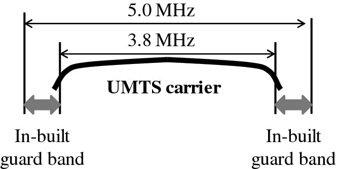
Figure 11.31 UMTS chip rate of 3.84 Mcps compared to nominal carrier spacing of 5.0 MHz
Figure 11.32 shows a spectrum migration example where the operator has in total 11.4 MHz. That would be the case with 900 MHz band with three operators: the total 900 MHz band is 35 MHz which leaves in practice 11.4 MHz per operator. The starting point is the GSM-only case with 57 GSM carriers. The UMTS refarming takes 4.2 MHz or 21 GSM carriers, which leaves 36 GSM carriers remaining. That GSM spectrum allows a high GSM capacity.
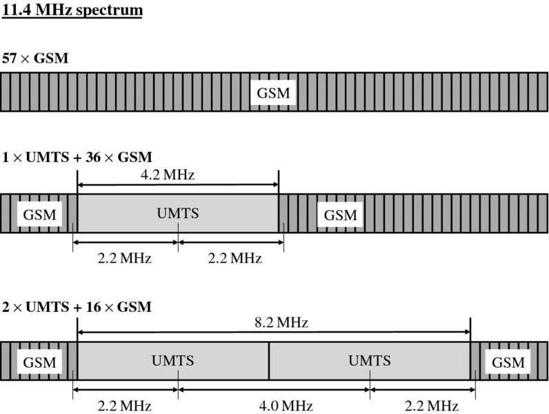
Figure 11.32 Example spectrum migration from GSM to UMTS
The second UMTS carrier can be deployed by using even less spectrum. The measurements show that 4.0 MHz separation between two WCDMA carriers can be used in practice, even 3.8 MHz spacing if some interference can be allowed between the two carriers. We assume 4.0 MHz spacing between two WCDMA carriers in Figure 11.32. The operator can still have 16 GSM carriers left after deploying dual-cell HSDPA at 900 MHz band. The combination of good coverage with low band and high data rate with dual-cell HSDPA brings a powerful radio solution.
11.6.3 GSM Features for Refarming
The UMTS refarming becomes smoother with the latest GSM features that improve the GSM spectrum efficiency: the same GSM traffic can be carried but with less spectrum. The most relevant GSM features are
- – Adaptive Multirate (AMR) voice coding, where the voice coding rate is changed between 4.75 kbps and 12.2 kbps according to the channel quality. Lower radio channel quality can be tolerated by using a lower data rate and more robust channel coding. Therefore, tighter frequency reuse can be applied in GSM by using AMR codec.
- – AMR half rate voice coding uses every second frame for the transmission, which can double the voice capacity and reduce the interference levels.
- – Orthogonal Subchannelization (OSC) allows packing even four users per time slot. The solution is to transmit to two users simultaneously and to separate the transmissions by interference cancellation receivers.
- – Dynamic Frequency and Channel Allocation (DFCA) uses time synchronized base stations where the Base Station Controller (BSC) allocates slots in time and frequency dimensions so that the inter-cell interference is minimized.
Using all these features can improve the GSM spectral efficiency by more than a factor of four. It is possible to squeeze down the GSM spectrum requirement considerably while still carrying good levels of GSM traffic. Most of the existing terminals in the field support these GSM features, which makes the practical deployment of these features easy.
11.6.4 Antenna Sharing Solutions
The preferable base station site solution utilizes the same antenna both for GSM and for UMTS in order to minimize the number of required physical antennas. Figure 11.33 shows the antenna sharing options. Option (a) uses so-called “over the air combining” where different antenna branches are used for GSM and UMTS. The dual cross-polarized antenna includes in total four ports: two for GSM and two for UMTS. The antenna width is slightly larger than the normal cross-polarized antenna. The benefit of option (a) is that UMTS can be deployed without any changes to GSM and there are no losses in the combining. Option (b) uses cross-polarized antenna and RF combining of GSM and UMTS signals. The in-band RF combining would normally cause some losses, but one option is to use one antenna branch for GSM and another for UMTS without any losses. Such a configuration is possible if MIMO is not used in UMTS and if only one carrier is used in GSM. Option (c) is the most advanced sharing solution with a single RF unit in the base station supporting both GSM and UMTS at the same time. This solution is called RF sharing and it is becoming the typical solution in network modernization cases.
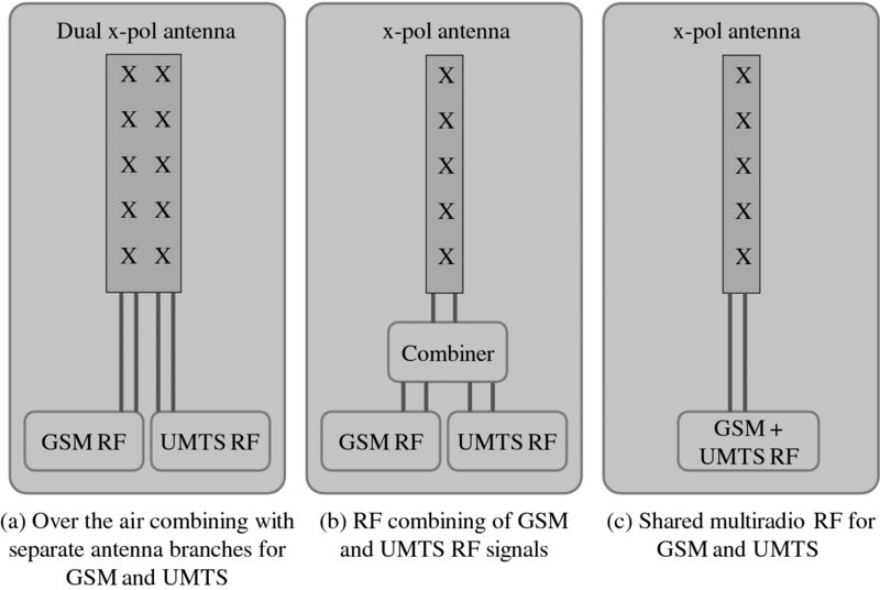
Figure 11.33 Antenna sharing options for GSM and UMTS
11.7 Summary
In this chapter we reviewed various topics covering key network deployment and dimensioning aspects.
Below are a summary of some of the most relevant considerations discussed:
- HSPA+ networks are typically limited in interference, and special care needs to be taken to control the amount of power transmitted in the network. Lack of coverage should be compensated with different solutions depending on the type of network – urban (typically limited by interference) or suburban/rural (typically limited by power).
- Antenna tilts are a very important tool to configure and maintain RF performance; however downtilting is often abused as the only way to achieve interference containment. Other methods include reducing powers, or even eliminating unnecessary sectors that are not required.
- Multilayer configuration should be done carefully depending on the type of deployment scenario: hotspots or continuous coverage zones, single or multiband, and so on.
- In networks with heavy smartphone penetration there are unexpected bottlenecks at the cell level (uplink congestion) as well as the RNC level (signaling processing capacity).
- As GSM traffic is reduced it should be possible to repurpose that spectrum for HSPA+. New carriers can be allocated in blocks as low as 3.8 MHz.
References
- Chevallier, C., Brunner, C., Caravaglia, A. et al. (2006) WCDMA (UMTS) Deployment Handbook: Planning and Optimization Aspects, John Wiley & Sons, Ltd, Chichester.
- Qualcomm Engineering Services Group (ESG), “Aspects of HSUPA Network Planning”, Revision A (April 6, 2007) (updated Sept 2008).
- Viterbi, A.J., Viterbi, A.M., and Zehavi, E. (1994) Other-cell interference in cellular power-controlled CDMA. IEEE Transactions on Communications, 42(234), Part 3, 1501–1504.
- Holma, H. and Toskala, A. (2006) HSDPA/HSUPA for UMTS. High Speed Radio Access for Mobile Communications, 1st edn, John Wiley & Sons, Ltd, Chichester.
- Bi, Q. (2004) A Forward Link Performance Study of the 1xEV-DO Rev. 0 System Using Field Measurements and Simulations, Lucent Technologies.