
Chapter 6
Real-Time Stereo 3D Imaging Techniques
Lazaros Nalpantidis
Robotics, Vision and Machine Intelligence lab., Department of Mechanical and Manufacturing Engineering, Aalborg University Copenhagen, Denmark
6.1 Introduction
Stereo vision involves the simultaneous use of two vision sensors and leads to the recovery of depth. It is based on the principal, first utilized by nature, that two spatially differentiated views of the same scene provide enough information to enable perception of the depth of the portrayed objects. This fact was first realized by Sir Charles Wheatstone, about two centuries ago, who stated: “…the mind perceives an object of three dimensions by means of the two dissimilar pictures projected by it on the two retinae…” [1].
Calculating the depth of various points, or any other primitive, in a scene relative to the position of a camera, is one of the important tasks of computer and robot vision systems. The most common method for extracting depth information from intensity images is by means of a pair of synchronized camera images acquired by a stereo rig, as the ones shown in Figure 6.1. Matching pixels of one image to pixels of the second image (also known as the stereo correspondence problem) results in the so called disparity map [2]. Disparity is defined as the difference of the coordinates of a matched pixel in the two images, which is proportional to its depth value. For rectified stereo pairs, the vertical disparity is always zero and, as a result, a disparity map consists of the horizontal disparity values for the matched image pixels. Nevertheless, the accurate and efficient estimation of disparity maps is a long-standing issue for the computer vision community [3].
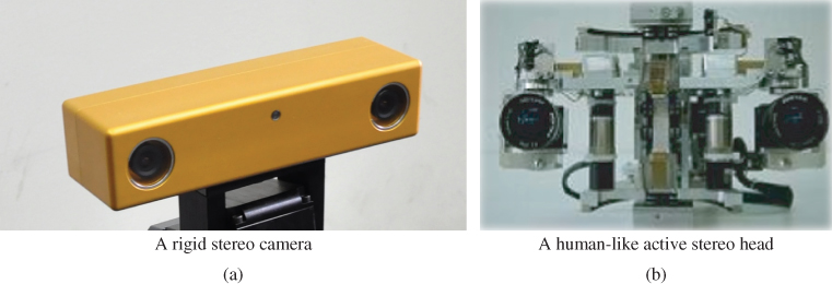
Figure 6.1 Stereo vision sensors.
The importance of stereo vision is apparent in the fields of machine vision [4], computer vision [5], virtual reality, robot navigation [6], simultaneous localization and mapping [7, 8], depth measurements [9] and 3D environment reconstruction [4]. The objective of this chapter is to provide a comprehensive survey of real-time stereo imaging algorithms and systems. The main characteristics of stereo vision algorithms are highlighted, with references to more detailed analyses where needed, and the state of the art concerning real-time implementations is given. The categorization followed in the rest of this Chapter follows the one shown in Figure 6.2.

Figure 6.2 Categorization of real-time stereo 3D imaging techniques.
6.2 Background
Even if stereo vision has been the focus of attention for many researchers during the past decades, it is still a very active and popular topic. The richness of the related literature and the number of newly published works every year reveal that there is room for improvement in the current state of the art. A consequence of this is that every attempt to capture the state of the art is destined to be outdated soon. However, what one can still deduce from the study of such surveys is the shift of focus and the new trends that arise over time.
Historically, the first attempts to gather, survey and compare stereo vision algorithms resulted in the review papers of Barnard and Fischler [10], Dhond and Aggarwal [11], and Brown [12]. However, the work that has had the biggest impact on the topic and defined clear directions is probably the seminal taxonomy and review paper of Scharstein and Szeliski [13]. In that work, apart from a detailed snapshot of the contemporary algorithms, a taxonomy framework, and an openly available objective test bench were proposed. The test bench consists a standard dataset of stereo images, metrics for evaluating the accuracy of the results, and also a website that hosts all the aforementioned, as well as an ever-updating list with the results of evaluated algorithms [14].
While the focus of Scharstein and Szeliski was the definition of a framework that would allow the computer vision community to pursue further accuracy of stereo algorithms, the rapid evolution of robotic applications and real-time vision systems in general, has indicated the execution speed as a factor of equal (if not greater) importance as the accuracy of the depth estimations. This trend is reflected and captured in subsequent reviews, such as in [15], in [16], where the branch of real-time hardware implementations is additionally covered, and in [17], where the focus is on real-time algorithms targeting resource-limited systems.
Apart from reviews and comparative presentations of complete stereo algorithms, there are also very useful works that compare the various alternatives for implementing each basic block of a stereo algorithm. As will be discussed in Section 3 of this chapter, the structure of stereo algorithms can be very well defined, and the various constituent parts can be clearly identified. Hirschmuller and Scharstein, in [18, 19] compare different (dis-)similarity measures (also referred to as matching cost functions) for local, semi-global, and global stereo algorithms.
Additionally, Gong and his colleagues, in [20], consider various alternatives for matching cost aggregation in real-time GPU-accelerated systems. Considering global methods for disparity assignment, Szeliski et al., in [21] propose some energy minimization benchmarks and use them to compare the quality of the results and the speed of several common energy minimization algorithms.
The stereo correspondence problem can be efficiently addressed by considering the geometry of the two stereo images and by applying image rectification to them. In the general case, the image planes of the two capturing cameras do not belong to the same plane. While stereo algorithms can deal with such cases, the demanded calculations are considerably simplified if the stereo image pair has been rectified. The process of rectification, as shown in Figure 6.3, involves the replacement of the initial image pair ![]() by another projectively equivalent pair
by another projectively equivalent pair ![]() [5, 2]. The initial images are reprojected on a common plane
[5, 2]. The initial images are reprojected on a common plane ![]() that is parallel to the baseline
that is parallel to the baseline ![]() joining the optical centers of the initial images.
joining the optical centers of the initial images.
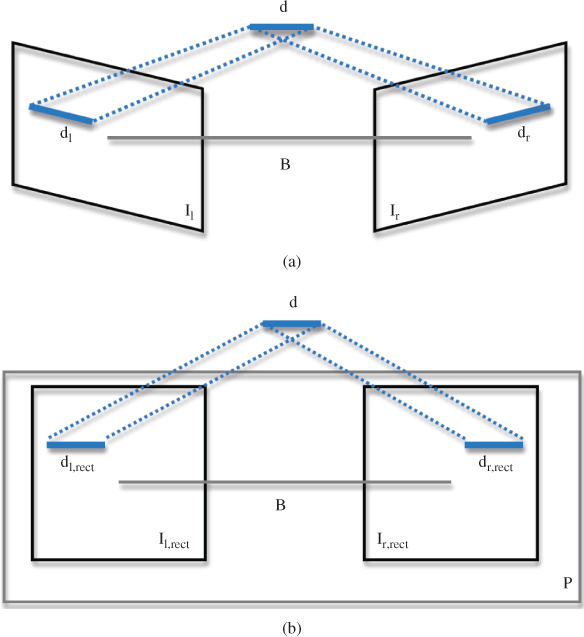
Figure 6.3 Rectification of a stereo pair. The two images  of an object
  (a) are replaced by two pictures
  that lie on a common plane
  (b).
(b).
Epipolar geometry provides tools in order to solve the stereo correspondence problem, i.e., to recognize the same feature in both images. If no rectification is performed, the matching procedure involves searching within two-dimensional regions of the target image. However, this matching can be done as a one-dimensional search, if accurately rectified stereo pairs are assumed in which horizontal scan lines reside on the same epipolar line, as shown in Figure 6.4. A point ![]() in one image plane may have arisen from any of points in the line C1P1, and may appear in the alternate image plane at any point on the epipolar line
in one image plane may have arisen from any of points in the line C1P1, and may appear in the alternate image plane at any point on the epipolar line ![]() [4]. Thus, the search is theoretically reduced within a scan line, since corresponding pair points reside on the same epipolar line. The difference of the horizontal coordinates of these points is the disparity value. The disparity map consists of all the disparity values of the image.
[4]. Thus, the search is theoretically reduced within a scan line, since corresponding pair points reside on the same epipolar line. The difference of the horizontal coordinates of these points is the disparity value. The disparity map consists of all the disparity values of the image.
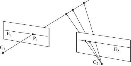
Figure 6.4 Geometry of epipolar lines, where  and
and  are the left and right camera lens centers, respectively. (a) Point
  in one image plane may have arisen from any of the points in the line
  , and may appear in the alternate image plane at any point on the epipolar line
  .
.
6.3 Structure of Stereo Correspondence Algorithms
The majority of the reported stereo correspondence algorithms can be described using more or less the same structural set [13]. The basic building blocks are the following:
- Computation of a matching cost function for every pixel in both the input images.
- Aggregation of the computed matching cost inside a support region for every pixel and every potential disparity value.
- Finding the optimum disparity value for every pixel of one picture.
- Refinement of the resulted disparity map.
Every stereo correspondence algorithm makes use of a matching cost function, so as to establish correspondence between two pixels, as discussed in Section 6.3.1. The results of the matching cost computation comprise the Disparity Space Image (DSI). DSI can be visualized as a 3D matrix containing the computed matching costs for every pixel and for all its potential disparity values [22]. The structure of a DSI is illustrated in Figure 6.5.

Figure 6.5 DSI containing matching costs for every pixel of the image and for all its potential disparity values.
Usually, the matching costs are aggregated over support regions. These regions could be 2D or even 3D [23, 24] ones within the DSI cube. The selection of the appropriate disparity value for each pixel is performed afterwards. It can be a simple Winner-Takes-All (WTA) process or a more sophisticated one. In many cases, this is an iterative process, as depicted in Figure 6.6. An additional disparity refinement step is frequently adopted. It is usually intended to filter the calculated disparity values, to give sub-pixel accuracy, or to assign values to not calculated pixels. The general structure of the majority of stereo correspondence algorithms is shown in Figure 6.6. Each block is discussed in more detailed in the rest of this section.

Figure 6.6 General structure of a stereo correspondence algorithm.
6.3.1 Matching Cost Computation
Detecting conjugate pairs in stereo images is a challenging research problem known as the correspondence problem, i.e., to find for each pixel in the left image the corresponding pixel in the right one [25]. The pixel to be matched without any ambiguity should be distinctly different from its surrounding pixels. To determine that two pixels form a conjugate pair, it is necessary to measure the similarity of these pixels, using some kind of a matching cost function. Among the most common ones are the absolute intensity differences (AD), the squared intensity differences (SD), and the normalized cross correlation (NCC). Evaluation of various matching costs can be found in [13, 18, 26].
AD is the simplest measure of all. It involves simple subtractions and calculations of absolute values. As a result, it is the most commonly used measure found in literature. The mathematical formulation of AD is:
where ![]() and
and ![]() denote the intensity values for the left and right image respectively,
denote the intensity values for the left and right image respectively, ![]() is the value of the disparity under examination ranging from 0 to
is the value of the disparity under examination ranging from 0 to ![]() and
and ![]() are the coordinates of the pixel on the image plane.
are the coordinates of the pixel on the image plane.
SD is somewhat more accurate in expressing the dissimilarity of two pixels. However, the higher computational cost of calculating the square of the intensities difference is not usually justified by the accuracy gain. It can be calculated as:
The normalized cross correlation calculates the dissimilarity of image regions instead of single pixels. It produces very robust results, on the cost of computational load. Its mathematical expression is:
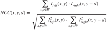
where ![]() is the image region under consideration.
is the image region under consideration.
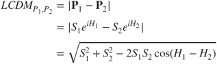
The luminosity-compensated dissimilarity measure (LCDM), as introduced in [27], provides stereo algorithms with tolerance to difficult lighting conditions. The images are initially transformed from the RGB to the HSL colorspace. The HSL colorspace inherently expresses the lightness of a color and demarcates it from its qualitative characteristics [28]. That is, an object will result in the same values of H and S regardless of the environment's illumination conditions. According to this assumption, LCDM disregards the values of the L channel in order to calculate the dissimilarity of two colors. The omission of the vertical (L) axis from the colorspace representation leads to a 2D circular disk, defined only by H and S. Thus, any color can be described as a planar vector with its initial point being the disk's center. As a consequence, each color ![]() can be described as a polar vector or, equivalently, as a complex number with modulus equal to
can be described as a polar vector or, equivalently, as a complex number with modulus equal to ![]() and argument equal to
and argument equal to ![]() . As a result, the difference, or equivalently the luminosity-compensated dissimilarity measure (LCDM), of two colors
. As a result, the difference, or equivalently the luminosity-compensated dissimilarity measure (LCDM), of two colors ![]() and
and ![]() can be calculated as the difference of the two complex numbers:
can be calculated as the difference of the two complex numbers:
On the other hand, the rank transform replaces the intensity of a pixel with its rank among all pixels within a certain neighborhood, and then calculates the absolute difference between possible matches [29]. Another matching cost used for pixel correlation is Mutual Information. This can express how similar two parts of an image are by calculating and evaluating the entropies of the joint and the individual probability distributions. The probability distributions are derived from the histograms of the corresponding image parts. Finally, there are also phase-based methods that treat images as signals and perform matching of some phase-related function.
A useful review and evaluation of various matching costs for establishing pixel correlation can be found in [19].
6.3.2 Matching Cost Aggregation
Usually, the matching costs are aggregated over support regions. Those support regions, often referred to as support or aggregating windows, could be square or rectangular, of fixed size or adaptive ones. The aggregation of the aforementioned cost functions leads to the core of most of the stereo vision methods, which can be mathematically expressed as follows, for the case of the sum of absolute differences (SAD):
And for the case of the sum of squared differences (SSD):
where ![]() are the intensity values in the left and right image,
are the intensity values in the left and right image, ![]() are the pixel's coordinates,
are the pixel's coordinates, ![]() is the disparity value under consideration and
is the disparity value under consideration and ![]() is the aggregated support region.
is the aggregated support region.
More sophisticated aggregation is traditionally considered as time-consuming. Methods based on extended local methodologies sacrifice some of their computational simplicity in order to obtain more accurate results [30]. Methods based on adaptive support weights (ASW) [31, 32] achieved this by using fixed-size support windows whose pixels' contribution in the aggregation stage varies, depending on their degree of correlation to the windows' central pixel. Despite the acceptance that these methods have enjoyed, the determination of a correlation function is still an open topic.
An ASW-based method for correspondence search is presented in [31]. The support-weights of the pixels in a given support window are adjusted based on color similarity and geometric proximity to reduce the image ambiguity. A similar approach is also adopted in [27], where stereo vision in non-ideal lighting conditions is examined, and in [33], where a psychophysically inspired stereo algorithm is presented.
On the other hand, some matching cost functions do not need an additional aggregation step, since this is an integral part of the cost calculation. As an example, the NCC and the rank transform require the a priori definition of a region where they are to be calculated.
An in-depth review and evaluation of different matching cost aggregation methods, suitable for implementation in programmable GPUs and for use in real-time systems can be found in [20].
6.4 Categorization of Characteristics
As already mentioned, there are numerous papers about stereo vision algorithms and systems published every year. This ever-growing list needs to be categorized according to some meaningful criteria to become tractable. Traditionally, the most common characteristics to divide the stereo algorithms literature has been the density of the computed disparity maps and the strategy used for the final assignment of disparity values. The rest of this Section examines the classes of such a categorization and discusses some indicative algorithms.
6.4.1 Depth Estimation Density
Stereo correspondence algorithms can be grouped into two broad groups; those producing dense and those producing sparse results. A dense stereo algorithm does not necessarily have to obtain disparity estimation for every single pixel. In practice, it is often impossible to achieve 100% density, due to occlusions in the stereo pair (even if certain techniques allow information propagation to such areas). As a result, the borderline between dense and sparse algorithms can be drawn depending on whether they actually attempt to match all the pixels, or only focus on a certain subset of them.
6.4.1.1 Dense
As more computational power becomes available in vision systems, dense stereo algorithms become more and more popular. Nowadays, published works about dense algorithms are dominating the relevant literature. Apart from the availability of the required computational resources, another factor that has boosted this class of algorithms is the existence of a standard test bench for the evaluation and objective comparison of their results accuracy. Thus, contemporary research in stereo matching algorithms, in accordance with the ideas of Maimone and Shafer [34], is reigned by the online tool available at the site maintained by Scharstein and Szeliski [13, 14]. The website provides a common dataset, and the produced disparity maps can be uploaded, automatically evaluated and listed together with the evaluation results, for ease of comparison.
As discussed already, not every pixel of one image has a corresponding one in its stereo pair image, mainly due to occlusions. However, algorithms that apply some kind of global optimization or “hole filling” mechanism can provide 100% coverage. In [35], an algorithm based on a hierarchical calculation of a mutual information-based matching cost is proposed. Its goal is to minimize a proper global energy function, not by iterative refinements, but by aggregating matching costs for each pixel from all directions. The final disparity map is sub-pixel accurate and occlusions are detected. The processing speed for the Teddy image set is 0.77 fps. The error in non-noccluded regions is found to be less than 3% for all the standard image sets. Calculations are made on an Intel Xeon processor running at 2.8 GHz.
An enhanced version of the previous method is proposed by the same author in [36]. Mutual information is, once again, used as cost function. The extensions applied in it result in intensity-consistent disparity selection for untextured areas and discontinuity-preserving interpolation for filling holes in the disparity maps. It treats successfully complex shapes and uses planar models for untextured areas. Bidirectional consistency check and sub-pixel estimation, as well as invalid disparities interpolation, are also performed. The experimental results indicate that the percentages of bad matching pixels in non-noccluded regions are 2.61, 0.25, 5.14 and 2.77 for the Tsukuba, Venus, Teddy and Cones image sets, respectively, with 64 disparity levels searched each time. However, the reported running speed on a 2.8 GHz PC is less than 1 fps.
6.4.1.2 Sparse
Sparse stereo algorithms provide depth estimations for only a limited subset of all the image pixels. The sparse disparity map is produced either by extracting and matching distinctive image features, or by filtering out the results of a dense method according to some reliability measure. In many cases, they stem from human vision studies and are based on matching for example segments or edges between two images.
Algorithms resulting in sparse, or semi-dense, disparity maps tend to be less attractive, as most of the contemporary applications require dense disparity information. However, they are very useful when:
- very rapid execution times are demanded;
- detail in the whole image is not required;
- reliability of the obtained depth estimations is more important than density.
Commonly, these types of algorithms tends to focus on striking characteristics of the images, leaving occluded and poorly textured areas unmatched. Veksler, in [37], presents an algorithm that detects and matches dense features between the left and right images of a stereo pair, producing a semi-dense disparity map. A dense feature is a connected set of pixels in the left image and a corresponding set of pixels in the right image, such that the intensity edges on the boundary of these sets are stronger than their matching error. All of these are computed during the stereo matching process. The algorithm computes disparity maps, with 14 disparity levels for the Tsukuba pair producing 66% density and 0.06% average error in the non-occluded regions.
Another method developed by Veksler [38] is based on the same basic concepts as the former one. The main difference is that this one uses the graph cuts algorithm for the dense feature extraction. As a consequence, this algorithm produces semi-dense results, with significant accuracy in areas where features are detected. The results are significantly better, considering density and error percentage, but they require longer running times. For the Tsukuba pair, it achieves a density up to 75%, the total error in the non-occluded regions is 0.36% and the running speed is 0.17 fps. For the Sawtooth pair, the corresponding results are 87%, 0.54% and 0.08 fps. All the results are obtained from a Pentium III PC running at 600 MHz; thus, significant speedup can be expected using a more powerful computer system.
In [39], a sparse stereo algorithm is initialized by extracting interesting points using the Harris corner detector. These points are used to construct a graph, and then the labeling problem is solved minimizing a global energy by means of graph cuts. Furthermore, a robust illumination changes structure tensor descriptor is used as similarity measurement to obtain even more accurate results.
More recently, Schauwecker et al., in [40], have incorporated a modified version of the very efficient FAST feature detector within a sparse stereo-matching algorithm. An additional consistency check filters out possible mismatches, and the final implementation can achieve processing rates above 200 fps on a simple dual core CPU computer platform.
6.4.2 Optimization Strategy
Stereo matching algorithms can be divided in three general classes, according to the way they assign disparities to pixels. First, there are algorithms that decide the disparity of each pixel according to the information provided by its local, neighboring pixels – thus called local or area-based methods. They are also referred to as window-based methods, because disparity computation at a given point depends only on intensity values within a finite support window. Second, there are algorithms that assign disparity values to each pixel, depending on information derived from the whole image – thus called global algorithms. These are also sometimes referred to as energy-based algorithms, because their goal is to minimize a global energy function, which combines data and smoothness terms, taking into account the whole image. Finally, the family of algorithms called semi-global select disparity values minimizing an energy function along scan-lines [41]. Of course, there are many other methods [42] that are not strictly included in either of these broad classes. The issue of stereo matching has recruited a variation of computation tools. Advanced computational intelligence techniques are not uncommon and constitute interesting and promiscuous directions [43, 44].
6.4.2.1 Local
After the computation and aggregation (if necessary) of matching costs, the actual selection of the best candidate matching pixel (and, thus, disparity value) has to be performed. Most local algorithms just choose the candidate match that exhibits the minimum matching cost. This simple winner-takes-all approach is very efficient in computational terms, but is also often inaccurate, resulting in faulty and incoherent disparity values.
Ogale and Aloimonos, in [45–47], propose a compositional approach to unify many early visual modules, such as segmentation, shape and depth estimation, occlusion detection, and local signal processing. The dissimilarity measure used is the phase differences from various frequency channels. As a result, this method can process images with contrast, among other mismatches.
6.4.2.2 Global
Contrary to local methods, global ones produce very accurate results at the expense of computation time. They formalize the disparity assignment step as a labeling problem, and their goal is to find the optimum disparity function ![]() that minimizes a global cost function
that minimizes a global cost function ![]() which combines data and smoothness terms.
which combines data and smoothness terms.
where ![]() takes into consideration the
takes into consideration the ![]() pixel's value throughout the image,
pixel's value throughout the image, ![]() provides the algorithm's smoothening assumptions and
provides the algorithm's smoothening assumptions and ![]() is a weight factor.
is a weight factor.
The minimization of the energy function is performed using a suitable iterative algorithm. Commonly used such algorithms include, among others, graph cuts [48, 49] and loopy belief propagation [50]. However, the main disadvantage of the global methods is that they are more time-consuming and computationally demanding.
An informative review and comparison of various energy minimization methods for global stereo matching can be found in [21].
6.4.2.3 Semi-global
The most popular semi-global stereo algorithms are based on Dynamic Programming (DP). DP has been used widely as an optimization method for the estimation of disparity ![]() along image scanlines [41, 51], and this is the reason for being called semi-global. The general idea behind a DP stereo algorithm is to treat the correspondence problem again as an energy minimization problem, but limited on scanlines. Thus, an energy function is formulated, again as in Equation 6.7, where the smoothness term can be formulated to handle depth discontinuities and occlusions along each scanline.
along image scanlines [41, 51], and this is the reason for being called semi-global. The general idea behind a DP stereo algorithm is to treat the correspondence problem again as an energy minimization problem, but limited on scanlines. Thus, an energy function is formulated, again as in Equation 6.7, where the smoothness term can be formulated to handle depth discontinuities and occlusions along each scanline.
DP stands somewhere between local and global algorithms, providing good accuracy of results in acceptable frame rates. Moreover, recent advances in DP-based stereo algorithms seem to be able to significantly improve both of these two aspects. Hardware implementations of DP have been reported [52, 53] that provide high execution speeds. Additionally, the incorporation of adaptive support weight aggregation schemes has been shown to further improve the accuracy and detail of the produced depth maps [54].
6.5 Categorization of Implementation Platform
Many stereo vision algorithms can achieve real-time or near-real-time operation. Such execution speeds can be obtained either by optimizing local stereo algorithms, or by employing custom hardware for speeding up the computations. In this section, implementations based on central processing unit (CPU), graphics processing unit (GPU), as well as field-programmable gate array (FPGA), or application-specific integrated circuits (ASIC), are covered that can be used in real-time systems.
6.5.1 CPU-only Methods
Gong and Yang, in [55], propose a reliability-based dynamic programming (RDP) algorithm that uses a different measure to evaluate the reliabilities of matches. According to this, the reliability of a proposed match is the cost difference between the globally best disparity assignment that includes the match and the one that does not include it. The inter-scanline consistency problem, common to the DP algorithms, is reduced through a reliability thresholding process. The result is a semi-dense unambiguous disparity map, with 76% density, 0.32% error rate and 16 fps for the Tsukuba, and 72% density, 0.23% error rate and 7 fps for the Sawtooth image pair. Accordingly, the results for Venus and Map pairs are 73%, 0.18%, 6.4 fps and 86%, 0.7%, 12.8 fps. As a result, the reported execution speeds, tested on a 2 GHz Pentium 4 PC, are encouraging for real-time operation if a semi-dense disparity map is acceptable.
Tombari et al. [56] present a local stereo algorithm that maximizes the speed-accuracy trade-off by means of an efficient segmentation-based AD cost aggregation strategy. The reported processing speed for the Tsukuba image pair is 5 fps and 1.7 fps for the Teddy and Art stereo image pairs.
Finally, in [57], a local stereo matching algorithm that computes dense disparity maps in real-time is presented. Two sizes for the used support windows improve the accuracy of the underlying SAD core, while keeping the computational cost low.
6.5.2 GPU-accelerated Methods
The active use of a GPU on a computer system can significantly improve execution speeds by exploiting the capabilities of GPUs to parallelize computations.
A hierarchical disparity estimation algorithm implemented on programmable 3D graphics processing unit (GPU) is reported in [58]. This method can process either rectified or uncalibrated image pairs. Bidirectional matching is utilized in conjunction with a locally aggregated sum of absolute intensity differences. This implementation on an ATI Radeon 9700 Pro can achieve up to 50 fps for ![]() pixel input images.
pixel input images.
In [59], a GPU implementation of a stereo algorithm that is able to achieve real-time performance with 4839 Millions of Disparity Estimation per Second (MDE/s) is presented. Highly accurate results are obtained, using a modified version of the SSD and filtering the results with a reliability criterion in the matching decision rule.
Kowalczuk and his colleagues, in [60], present a real-time stereo matching method that uses a two-pass approximation of adaptive support-weight aggregation and a low-complexity iterative disparity refinement technique. The implementation on a programmable GPU using CUDA is able to achieve 152.5 MDE/s, resulting in 62 fps for ![]() images with 32 disparity levels.
images with 32 disparity levels.
The work of Richardt et al. [61] proposes a variation of Yoon and Kweon's [31] algorithm, implemented on a GPU. The implementation can achieve more than 14 fps, retaining the high quality of the original algorithm.
An algorithm that generates high quality results in real time is reported in [62]. It is based on the minimization of a global energy function. The hierarchical belief propagation algorithm iteratively optimizes the smoothness term, but achieves fast convergence by removing redundant computations involved. In order to accomplish real-time operation, the authors take advantage of the parallelism of a GPU. Experimental results indicate 16 fps processing speed for ![]() pixel self-recorded images with 16 disparity levels. The percentages of bad matching pixels in non-occluded regions for the Tsukuba, Venus, Teddy and Cones image sets are found to be 1.49, 0.77, 8.72 and 4.61. The computer used is a 3 GHz PC and the GPU is an NVIDIA GeForce 7900 GTX graphics card with 512M video memory.
pixel self-recorded images with 16 disparity levels. The percentages of bad matching pixels in non-occluded regions for the Tsukuba, Venus, Teddy and Cones image sets are found to be 1.49, 0.77, 8.72 and 4.61. The computer used is a 3 GHz PC and the GPU is an NVIDIA GeForce 7900 GTX graphics card with 512M video memory.
Additionally, another GPU implementation of a global stereo algorithm based on hierarchical belief propagation is presented in [63]. An approximate disparity map calculation or motion estimation, in higher levels, is used to limit the search space without significantly affecting the accuracy of the obtained results.
Wang et al., in [54], present a stereo algorithm that combines high quality results with real-time performance. DP is used in conjunction with an adaptive aggregation step. The per-pixel matching costs are aggregated in the vertical direction only, resulting in improved inter-scanline consistency and sharp object boundaries. This work exploits the color and distance proximity-based weight assignment for the pixels inside a fixed support window, as reported in [31]. The real-time performance is achieved due to the parallel use of the CPU and the GPU of a computer. This implementation can process ![]() pixel images with 16 disparity levels at 43.5 fps, and
pixel images with 16 disparity levels at 43.5 fps, and ![]() pixel images with 16 disparity levels at 9.9 fps. The test system is a 3.0 GHz PC with an ATI Radeon XL1800 GPU.
pixel images with 16 disparity levels at 9.9 fps. The test system is a 3.0 GHz PC with an ATI Radeon XL1800 GPU.
Finally, a near-real-time stereo matching technique is presented in [64], which is based on the RDP algorithm. This algorithm can generate semi-dense disparity maps. Two orthogonal RDP passes are used to search for reliable disparities along both horizontal and vertical scanlines. Hence, the inter-scanline consistency is explicitly enforced. It takes advantage of the computational power of programmable graphics hardware, which further improves speed. The algorithm is tested on an Intel Pentium 4 computer running at 3 GHz, with a programmable ATI Radeon 9800 XT GPU equipped with 256MB video memory. It results in 85% dense disparity map with 0.3% error rate at 23.8 fps for the Tsukuba pair, 93% density, 0.24% error rate at 12.3 fps for the Sawtooth pair, 86% density, 0.21% error rate at 9.2 fps for the Venus pair and 88% density, 0.05% error rate at 20.8 fps for the Map image pair. If needed, the method can also be used to generate more dense disparity maps, deteriorating the execution speed.
6.5.3 Hardware Implementations (FPGAs, ASICs)
The use of dedicated and specifically designed hardware for the implementation of stereo algorithms can really boost their performance. However, not all stereo algorithms are easy to implement efficiently in hardware [16]. Furthermore, the effort and time required for such implementations are significant, while further changes are difficult to incorporate.
The FPGA-based system developed by [65] is able to compute dense disparity maps in real time, using the SAD method over fixed windows. The whole algorithm, including radial distortion correction, Laplacian of Gaussian (LoG) filtering, correspondence finding, and disparity map computation, is implemented in a single FPGA. The system can process ![]() pixel images with 64 disparity levels and 8-bit depth precision at 30 fps speed, and
pixel images with 64 disparity levels and 8-bit depth precision at 30 fps speed, and ![]() pixel images at 50 fps.
pixel images at 50 fps.
On the other hand, a slightly more complex implementation than the previous one is proposed in [66]. It is based on the SAD using adaptive sized windows. The proposed method iteratively refines the matching results by hierarchically reducing the window size. The results obtained by the proposed method are 10% better than that of a fixed-window method. The architecture is fully parallel and, as a result, all the pixels and all the windows are processed simultaneously. The speed for ![]() pixel images with 8-bit grayscale precision and 64 disparity levels is 30 fps. The resources consumption is 42.5K logic elements, i.e. 82% of the considered FPGA device.
pixel images with 8-bit grayscale precision and 64 disparity levels is 30 fps. The resources consumption is 42.5K logic elements, i.e. 82% of the considered FPGA device.
SAD aggregated using adaptive windows is the core of the work presented in [67]. A hardware-based CA parallel-pipelined design is realized on a single FPGA device. The achieved speed is nearly 275 fps, for ![]() pixel image pairs with a disparity range of 80 pixels. The presented hardware-based algorithm provides very good processing speed at the expense of accuracy. The device utilization is 149K gates, that is 83% of the available resources.
pixel image pairs with a disparity range of 80 pixels. The presented hardware-based algorithm provides very good processing speed at the expense of accuracy. The device utilization is 149K gates, that is 83% of the available resources.
The work of [52] implement an SAD algorithm on a FPGA board featuring external memory and a Nios II embedded processor clocked at 100 MHz. The implementation produces dense 8-bit disparity maps of ![]() pixels with 32 disparity levels at a speed of 14 fps. Essential resources are about 16K logic elements whereas, by migrating to more complex devices, the design can be scaled up to provide better results.
pixels with 32 disparity levels at a speed of 14 fps. Essential resources are about 16K logic elements whereas, by migrating to more complex devices, the design can be scaled up to provide better results.
The same authors, in [53], present an improved SAD-based algorithm with a fixed ![]() aggregation window and a hardware median enhancement filter. The presented system can process
aggregation window and a hardware median enhancement filter. The presented system can process ![]() images with 64 disparity levels at 162 fps speed. The implementation requires 32K logic elements, equivalent to about 63K gates.
images with 64 disparity levels at 162 fps speed. The implementation requires 32K logic elements, equivalent to about 63K gates.
The work of Ambrosch and Kubinger in [68] presents an FPGA implementation of a local stereo algorithm. The algorithm combines the use of gradient-based census transform with adaptive support window SAD. The implementation is able to process ![]() pixel images at 60 fps.
pixel images at 60 fps.
Zicari et al., in [69], implemented a SAD algorithm with an additional consistency check on an FPGA. The algorithm can process ![]() grayscale images with 30 disparity levels at 97 fps.
grayscale images with 30 disparity levels at 97 fps.
Furthermore, the work of Kostavelis et al. [70] includes a FPGA implementation of a dense SAD-based stereo algorithm, as part of a vision system for planetary autonomous robots. The implementation on a Xilinx Virtex 6 FPGA device can process ![]() images, with 200 disparity level and quarter-pixel accuracy in 0.59 fps, which is found to be more than sufficient for the needs of the considered space exploratory rover.
images, with 200 disparity level and quarter-pixel accuracy in 0.59 fps, which is found to be more than sufficient for the needs of the considered space exploratory rover.
The use of DP has been explored as well. The implementation presented in [71] uses the DP search method on a trellis solution space. It can cope with the case of vergent cameras, i.e., cameras with optical axes that intersect. The images received from a pair of cameras are rectified using linear interpolation, and then the disparity is calculated. The architecture has the form of a linear systolic array, using simple processing elements. The design is canonical and simple to be implemented in parallel. The implementation requires 208 processing elements and the resulting system can process ![]() pixel images with up to 208 disparity levels at 15 fps.
pixel images with up to 208 disparity levels at 15 fps.
An extension of the previous method is presented in [72]. The main difference is that data from the previous line are incorporated, so as to enforce better inter-scanline inconsistency. The running speed is 30 fps for ![]() pixel images with 128 disparity levels. The number of utilized processing elements is 128. The percentage of pixels with disparity error larger than 1 in the non-noccluded areas is 2.63, 0.91, 3.44 and 1.88 for the Tsukuba, Map, Venus and Sawtooth image sets, respectively.
pixel images with 128 disparity levels. The number of utilized processing elements is 128. The percentage of pixels with disparity error larger than 1 in the non-noccluded areas is 2.63, 0.91, 3.44 and 1.88 for the Tsukuba, Map, Venus and Sawtooth image sets, respectively.
Finally, the work of [53] also presents a custom parallelized DP algorithm. Once again, a fixed ![]() aggregation window and a hardware median enhancement filter is used. Moreover, inter-scanline support is utilized. The presented system can process
aggregation window and a hardware median enhancement filter is used. Moreover, inter-scanline support is utilized. The presented system can process ![]() images with 65 disparity levels at 81 fps speed. The implementation require 270K logic elements, equivalent to about 1.6M gates.
images with 65 disparity levels at 81 fps speed. The implementation require 270K logic elements, equivalent to about 1.6M gates.
The implementation of stereo algorithms on ASICs can result in very fast systems – even faster than when using FPGAs. However, this alternative is much more expensive, apart from the case of massive production. The prototyping times are considerable longer, and the result is highly process-dependent. Any further changes are difficult and, additionally, time- and money-consuming. As a result, the performance supremacy of ASIC implementations does not, in most cases, justify choosing them over the other possibilities. These are the main reasons that make recent ASIC implementation publications rare in contrast to the FPGA-based ones.
Published works concerning ASIC implementations of stereo matching algorithms [73, 74] are restricted to the use of SAD. The reported architectures make extensive use of parallelism and seem promising.
6.6 Conclusion
Stereo vision remains an attractive solution to the 3D imaging issue. This chapter has covered the basics of the theory behind stereo vision algorithms and has tried to categorize them according to their main characteristics and implementation platforms. A snapshot of the state of the art has been given.
One of the conclusions that can be deduced from this work is that the center of attention regarding stereo vision seems to have shifted; it is not only accuracy that is pursued, as it used to be, but also real-time performance that is now demanded. The solution to this issue is coming, either by simple algorithms implemented on powerful contemporary CPU systems, or by exploiting the power of programmable GPU co-processors, or by developing hardware-friendly implementations for FPGAs. The two latter options seem to be gaining popularity, as they can combine real-time execution speeds with very accurate depth estimations.
Another interesting observation is that local algorithms are not any more the only ones able to be implemented and executed in real time. Semi-global, or even purely global stereo algorithms, are reported to achieve acceptable frame rates. This trend seems to be growing, due to the fact that more powerful platforms are becoming constantly available, and more efficient and optimized versions of those algorithms are regularly being proposed.
The maturity of stereo vision techniques and their capability to operate in both indoor and outdoor environments give stereo vision a solid foundation in the harsh competition against other 3D sensing technologies. As a result, real-time implementations of stereo vision algorithms find their way in modern human-machine interaction systems, home entertainment systems, and autonomous robots, just to name a few.
References
- 1. Wheatstone, C. (1838). Contributions to the physiology of vision – part the first. on some remarkable, and hitherto unobserved, phenomena of binocular vision. Philosophical Transactions of the Royal Society of London, 371–394.
- 2. Faugeras, O. (1993). Three-dimensional computer vision: a geometric viewpoint. MIT Press, Cambridge.
- 3. Marr, D., Poggio, T. (1976). Cooperative computation of stereo disparity. Science 194(4262), 283–287.
- 4. Jain, R., Kasturi, R., Schunck, B.G. (1995). Machine vision. McGraw-Hill, New York, USA.
- 5. Forsyth, D.A., Ponce, J. (2002). Computer Vision: A modern Approach. Prentice Hall, Upper Saddle River, NJ, USA.
- 6. Metta. G, Gasteratos, A., Sandini, G. (2004). Learning to track colored objects with log-polar vision. Mechatronics 14(9), 989–1006.
- 7. Murray, D., Little, J.J. (2000). Using real-time stereo vision for mobile robot navigation. Autonomous Robots 8(2), 161–171.
- 8. Murray, D., Jennings, C. (1997). Stereo vision based mapping and navigation for mobile robots. IEEE International Conference on Robotics and Automation, 2, 1694–1699.
- 9 Manzotti, R., Gasteratos, A., Metta, G., Sandini, G. (2001). Disparity estimation on log-polar images and vergence control. Computer Vision and Image Understanding 83(2), 97–117.
- 10. Barnard, S.T., Fischler, M.A. (1982). Computational stereo. ACM Computing Surveys 14(4), 553–572.
- 11. Dhond, U.R., Aggarwal, J.K. (1989). Structure from stereo – a review. IEEE Transactions on Systems, Man, and Cybernetics 19(6), 1489–1510.
- 12. Brown, L.G. (1992). A survey of image registration techniques. Computing Surveys 24(4), 325–376.
- 13. Scharstein, D., Szeliski, R. (2002). A taxonomy and evaluation of dense two-frame stereo cor- respondence algorithms. International Journal of Computer Vision 47(1–3), 7–42.
- 14. http://vision.middlebury.edu/stereo/ (2010).
- 15. Sunyoto, H., van der Mark, W., Gavrila, D.M. (2004). A comparative study of fast dense stereo vision algorithms. IEEE Intelligent Vehicles Symposium, 319–324.
- 16. Nalpantidis, L., Sirakoulis, G.C., Gasteratos, A. (2008). Review of stereo vision algorithms: from software to hardware. International Journal of Optomechatronics 2(4), 435–462.
- 17. Tippetts, B., Lee, D.J., Lillywhite, K., Archibald, J. (2013). Review of stereo vision algorithms and their suitability for resource-limited systems. Journal of Real-Time Image Processing.
- 18. Hirschmuller, H., Scharstein, D. (2007). Evaluation of cost functions for stereo matching. IEEE Computer Society Conference on Computer Vision and Pattern Recognition, Minneapolis, Minnesota, USA.
- 19. Hirschmuller, H., Scharstein, D. (2009). Evaluation of stereo matching costs on images with radiometric differences. IEEE Transactions on Pattern Analysis and Machine Intelligence 31(9), 1582–1599.
- 20. Gong, M., Yang, R., Wang, L., Gong, M. (2007). A performance study on different cost aggregation approaches used in real-time stereo matching. International Journal of Computer Vision 75(2), 283–296.
- 21. Szeliski, R., Zabih, R., Scharstein, D., Veksler, O., Kolmogorov, V., Agarwala, A., Tappen, M., Rother, C. (2008). A comparative study of energy minimization methods for markov random fields with smoothness-based priors. IEEE transact. pattern anal. mach. intell. IEEE Transactions on Pattern Analysis and Machine Intelligence 30(6), 1068–1080.
- 22. Muhlmann, K., Maier, D., Hesser, J., Manner, R. (2002). Calculating dense disparity maps from color stereo images, an efficient implementation. International Journal of Computer Vision 47(1–3), 79–88.
- 23. Zitnick, C.L., Kanade, T. (2000). A cooperative algorithm for stereo matching and occlusion detection. IEEE Transactions on Pattern Analysis and Machine Intelligence 22(7), 675–684.
- 24. Brockers, R., Hund, M., Mertsching, B. (2005). Stereo vision using cost-relaxation with 3D support regions. Image and Vision Computing New Zealand, 96–101.
- 25. Barnard, S.T., Thompson, W.B. (1980). Disparity analysis of images. IEEE Transactions on Pattern Analysis and Machine Intelligence 2(4), 333–340.
- 26. Mayoral, R., Lera, G., Perez-Ilzarbe, M.J. (2006). Evaluation of correspondence errors for stereo. Image and Vision Computing 24(12), 1288–1300.
- 27. Nalpantidis, L., Gasteratos, A. (2010). Stereo vision for robotic applications in the presence of non-ideal lighting conditions. Image and Vision Computing 28, 940–951.
- 28. Gonzalez, R.C., Woods, R.E. (1992). Digital Image Processing. Addison-Wesley Longman Publishing Co, Inc, Boston, MA, USA.
- 29. Zabih, R., Woofill, J. (1994). Non-parametric local transforms for computing visual correspondence. European Conference of Computer Vision, 151–158.
- 30. Mordohai, P., Medioni, G.G. (2006). Stereo using monocular cues within the tensor voting framework. IEEE Transactions on Pattern Analysis and Machine Intelligence 28(6), 968–982.
- 31. Yoon, K.-J., Kweon, I.S. (2006). Adaptive support-weight approach for correspondence search. IEEE Transactions on Pattern Analysis and Machine Intelligence 28(4), 650–656.
- 32. Gu, Z., Su, X., Liu, Y., Zhang, Q. (2008). Local stereo matching with adaptive support-weight, rank transform and disparity calibration. Pattern Recognition Letters 29(9), 1230–1235.
- 33. Nalpantidis, L., Gasteratos, A. (2010). Biologically and psychophysically inspired adaptive support weights algorithm for stereo correspondence. Robotics and Autonomous Systems 58, 457–464.
- 34. Maimone, M.W., Shafer, S.A. (1996). A taxonomy for stereo computer vision experiments. ECCV Workshop on Performance Characteristics of Vision Algorithms, 59–79.
- 35. Hirschmuller, H. (2005). Accurate and efficient stereo processing by semi-global matching and mutual information. IEEE Computer Society Conference on Computer Vision and Pattern Recognition, 2, 807–814.
- 36. Hirschmuller, H. (2006). Stereo vision in structured environments by consistent semi-global matching. IEEE Computer Society Conference on Computer Vision and Pattern Recognition, 2, 2386–2393.
- 37 Veksler, O. (2002). Dense features for semi-dense stereo correspondence. International Journal of Computer Vision 47(1–3), 247–260.
- 38. Veksler, O. (2003). Extracting dense features for visual correspondence with graph cuts. IEEE Computer Vision and Pattern Recognition 1, 689–694.
- 39. Mu, Y., Zhang, H., Li, J. (2009). A global sparse stereo matching method under structure tensor constraint. International Conference on Information Technology and Computer Science, 1, 609–612.
- 40. Schauwecker, K., Klette, R., Zell, A. (2012). A new feature detector and stereo matching method for accurate high-performance sparse stereo matching. IEEE/RSJ International Conference on Intelligent Robots and Systems, 5171–5176.
- 41. Cox, I.J., Hingorani, S.L., Rao, S.B., Maggs, B.M. (1996). A maximum likelihood stereo algorithm. Computer Vision and Image Understanding 63, 542–567.
- 42. Liu, C., Pei, W., Niyokindi, S., Song, J., Wang, L. (2006). Micro stereo matching based on wavelet transform and projective invariance. Measurement Science and Technology 17(3), 565–571.
- 43. Binaghi, E., Gallo, I., Marino, G., Raspanti, M. (2004). Neural adaptive stereo matching. Pattern Recognition Letters 25(15), 1743–1758.
- 44. Kotoulas, L., Gasteratos, A., Sirakoulis, G.C., Georgoulas, C., Andreadis, I. (2005). enhancement of fast acquired disparity maps using a 1-D cellular automation filter. IASTED International Conference on Visualization, Imaging and Image Processing, Benidorm, Spain, 355–359.
- 45. Ogale, A.S., Aloimonos, Y. (2005). Robust contrast invariant stereo correspondence. IEEE International Conference on Robotics and Automation, 819–824.
- 46. Ogale, A.S., Aloimonos, Y. (2005). Shape and the stereo correspondence problem. International Journal of Computer Vision 65(3), 147–162.
- 47. Ogale, A.S., Aloimonos, Y. (2007). A roadmap to the integration of early visual modules. International Journal of Computer Vision 72(1), 9–25.
- 48. Boykov, Y., Veksler, O., Zabih, R. (2001). Fast approximate energy minimization via graph cuts. IEEE Transactions on Pattern Analysis and Machine Intelligence 23(11), 1222–1239.
- 49. Boykov, Y., Kolmogorov, V. (2001). An experimental comparison of min-cut/max-ow algo- rithms for energy minimization in vision. IEEE Transactions on Pattern Analysis and Machine Intelligence 26, 359–374.
- 50. Yedidia, J.S., Freeman, W., Weiss, Y. (2000). Generalized belief propagation. Conference on Neural Information Processing Systems, 689–695.
- 51. Bobick, A.F., Intille, S.S. (1999). Large occlusion stereo. International Journal of Computer Vision 33, 181–200.
- 52. Kalomiros, J.A., Lygouras, J. (2008). Hardware implementation of a stereo co-processor in a medium-scale field programmable gate array. IET Computers and Digital Techniques 2(5), 336–346.
- 53. Kalomiros, J., Lygouras, J. (2009). Comparative study of local SAD and dynamic programming for stereo processing using dedicated hardware. EURASIP Journal on Advances in Signal Processing 1–189.
- 54. Wang, L., Liao, M., Gong, M., Yang, R., Nister, D. (2006). High-quality real-time stereo using adaptive cost aggregation and dynamic programming. Third International Symposium on 3D Data Processing, Visualization, and Transmission, 798–805.
- 55. Gong, M., Yang, Y.–H. (2005). Fast unambiguous stereo matching using reliability-based dynamic programming. IEEE Transactions on Pattern Analysis and Machine Intelligence 27(6), 998–1003.
- 56. Tombari, F., Mattoccia, S., Di Stefano, L., Addimanda, E. (2008). Near real-time stereo based on effective cost aggregation. International Conference on Pattern Recognition, 1–4.
- 57. Gupta, R.K., Cho, S.-Y. (2010). A correlation-based approach for real-time stereo matching. International Symposium on Visual Computing, 6454, 129–138.
- 58. Zach, C., Karner, K., Bischof, H. (2004). Hierarchical disparity estimation with programmable 3D hardware. International Conference in Central Europe on Computer Graphics, Visualization and Computer Vision, 275–282.
- 59. Drazic, V., Sabater, N. (2012). A precise real-time stereo algorithm. 27th Conference on Image and Vision Computing New Zealand, 138–142.
- 60. Kowalczuk, J., Psota, E.T., Perez, L.C. (2013). Real-time stereo matching on cuda using an iterative refinement method for adaptive support-weight correspondences. IEEE Transactions on Circuits and Systems for Video Technology 23(1), 94–104.
- 61. Richardt, C., Orr, D., Davies, I., Criminisi, A., Dodgson, N. (2010). A. Real-time spatiotemporal stereo matching using the dual-cross-bilateral grid. European Conference on Computer Vision (ECCV), ser. Lecture Notes in Computer Science, 6313, 510–523.
- 62. Yang, Q., Wang, L., Yang, R. (2006). Real-time global stereo matching using hierarchical belief propagation. British Machine Vision Conference, 3, 989–998.
- 63 Grauer-Gray, S., Kambhamettu, C. (2009). Hierarchical belief propagation to reduce search space using cuda for stereo and motion estimation. Workshop on Applications of Computer Vision, 1–8.
- 64. Gong, M., Yang, Y.–H. (2005). Near real-time reliable stereo matching using programmable graphics hardware. IEEE Computer Society Conference on Computer Vision and Pattern Recognition, 1, 924–931.
- 65. Jia, Y., Xu, Y., Liu, W., Yang, C., Zhu, Y., Zhang, X., An, L. (2003). A miniature stereo vision machine for real-time dense depth mapping. International Conference on Computer Vision Systems, ser. Lecture Notes in Computer Science, 2626, 268–277.
- 66. Hariyama, M., Kobayashi, Y., Sasaki, H., Kameyama, M. (2005). FPGA implementation of a stereo matching processor based on window-parallel-and-pixel-parallel architecture. IEICE Transactions on Fundamentals of Electronics, Communications and Computer Science 88(12), 3516–3522.
- 67. Georgoulas, C., Kotoulas, L., Sirakoulis, G.C., Andreadis, I., Gasteratos, A. (2008). Real-time disparity map computation module Journal of Microprocessors and Microsystems 32(3), 159–170.
- 68. Ambrosch, K., Kubinger, W. (2010). Accurate hardware-based stereo vision. Computer Vision and Image Understanding 114(11), 1303–1316.
- 69. Zicari, P., Perri, S., Corsonello, P., Cocorullo, G. (2012). Low-cost FPGA stereo vision system for real time disparity maps calculation. Microprocessors and Microsystems 36(4), 281–288.
- 70. Kostavelis, I., Nalpantidis, L., Boukas, E., Rodrigalvarez, M., Stamoulias, I., Lentaris, G., Diamantopoulos, D., Siozios, K., Soudris, D., Gasteratos, A. (in press). SPARTAN: Developing a vision system for future autonomous space exploration robots. Journal of Field Robotics.
- 71. Jeong, H., Park, S. (2004). Generalized trellis stereo matching with systolic array. International Symposium on Parallel and Distributed Processing and Applications, 3358, 263–267. Springer Verlag.
- 72. Park, S., Jeong, H. (2007). Real-time stereo vision FPGA chip with low error rate. International Conference on Multimedia and Ubiquitous Engineering, 751–756.
- 73. Hariyama, M., Takeuchi, T., Kameyama, M. (2000). Reliable stereo matching for highly-safe intelligent vehicles and its VLSI implementation. IEEE Intelligent Vehicles Symposium, 128–133.
- 74. Hariyama, M., Sasaki, H., Kameyama, M. (2005). Architecture of a stereo matching VLSI processor based on hierarchically parallel memory access. IEICE Transactions on Information and Systems E88-D(7), 1486–1491.