
Chapter 22
Using Advanced 3D Features
The Autodesk® AutoCAD® 2014 software has an extended set of tools for working with 3D drawings that lets you create 3D objects with few limitations on shape and orientation. This chapter focuses on the use of these tools, which help you easily generate 3D forms and view them in both perspective and orthogonal modes.

The AutoCAD LT® software doesn’t support any of the features described in this chapter.
In this chapter, you will learn to:
- Master the User Coordinate System
- Understand the UCS options
- Use viewports to aid in 3D drawing
- Use the array tools
- Create complex 3D surfaces
- Create spiral forms
- Create surface models
- Move objects in 3D space
Setting Up AutoCAD for This Chapter
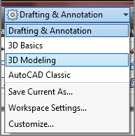
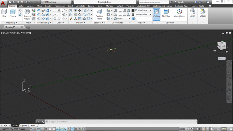
Before you start, we’d like you to set up AutoCAD in a way that will make your work a little easier. You’ll use the 3D Modeling workspace to which you were introduced in Chapter 21, “Creating 3D Drawings.” To do so, start AutoCAD, and then click the Workspace drop-down in the Quick Access toolbar and select 3D Modeling, as shown in Figure 22-1. You’ll see a new set of panels appear, as shown in Figure 22-2.
Figure 22-1 Select 3D Modeling from the Workspace drop-down.
In Chapter 21, you started a new 3D model using a template set up for 3D modeling. Here you’ll start to work with the default 2D drawing, acad.dwt. Now you’re ready to get to work.
Figure 22-2 The AutoCAD window set up for this chapter
Mastering the User Coordinate System
The User Coordinate System (UCS) enables you to define a custom coordinate system in 2D and 3D space. You’ve been using the default coordinate system called the World Coordinate System (WCS) all along. By now, you’re familiar with the L-shaped icon in the lower-left corner of the AutoCAD screen, containing a small square and the letters X and Y. The square indicates that you’re currently in the WCS; the X and Y indicate the positive directions of the x- and y-axes. The WCS is a global system of reference from which you can define other UCSs.
It may help to think of these AutoCAD UCSs as different drawing surfaces or two-dimensional planes. You can have several UCSs at any given time. By setting up these different UCSs, you can draw as you would in the WCS in 2D and still create a 3D image.
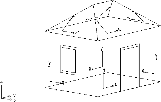
Suppose you want to draw a house in 3D with doors and windows on each of its sides. You can set up a UCS for each of the sides, and then you can move from UCS to UCS to add your doors and windows (see Figure 22-3). In each UCS, you draw your doors and windows as you would in a typical 2D drawing. You can even insert elevation views of doors and windows that you created in other drawings.
Figure 22-3 Different UCSs in a 3D drawing
In this chapter, you’ll experiment with several views and UCSs. All the commands you’ll use are available both at the command line and via the View tab’s Coordinates panel.
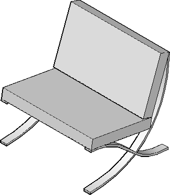
Defining a UCS
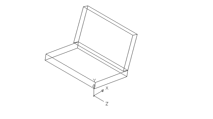
In the first set of exercises, you’ll draw a chair that you can later add to your 3D unit drawing. In drawing this chair, you’ll be exposed to the UCS as well as to some of the other 3D capabilities available in AutoCAD:
Figure 22-4 The chair seat and back in the Plan (top) and Isometric (bottom) views
Notice that the UCS icon appears in the same plane as the current coordinate system. The icon will help you keep track of which coordinate system you’re in. Now you can see the chair components as 3D objects.
Next you’ll define a UCS that is aligned with one side of the seat:
Figure 22-5 The UCS dialog box
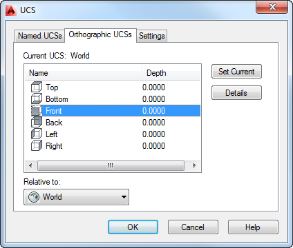
Figure 22-6 The six predefined UCS orientations
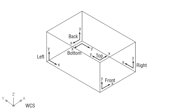
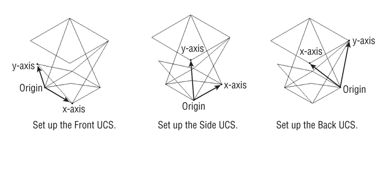
The Orthographic UCSs tab offers a set of predefined UCSs for each of the six standard orthographic projection planes. Figure 22-6 shows these UCSs in relation to the WCS.
Because a good part of 3D work involves drawing in these orthographic planes, AutoCAD supplies the ready-made UCS orientations for quick access. But you aren’t limited to these six orientations. If you’re familiar with mechanical drafting, you’ll see that the orthographic UCSs correspond to the typical orthographic projections used in mechanical drafting. If you’re an architect, the Front, Left, Back, and Right UCSs correspond to the south, west, north, and east elevations of a building.
Before you continue building the chair model, you’ll move the UCS to the surface on which you’ll be working. Right now, the UCS has its origin located in the same place as the WCS origin.
You can move a UCS so that its origin is anywhere in the drawing:
Figure 22-7 Setting up a UCS
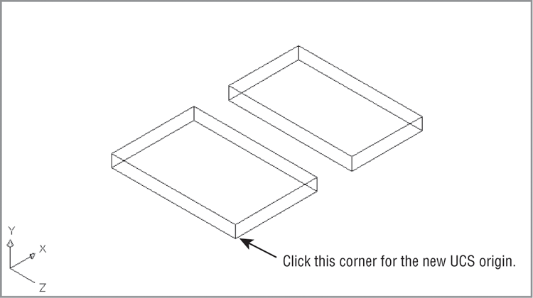
You just created a new UCS based on the Front UCS you selected from the UCS dialog box. Now, as you move your cursor, the origin of the UCS icon corresponds to a 0,0 coordinate. Although you have a new UCS, the WCS still exists; you can always return to it when you need to.
Saving a UCS
After you’ve gone through the work of creating a UCS, you may want to save it—especially if you think you’ll come back to it later. Here’s how to save a UCS:
Your UCS is now saved with the name 3DSW. You can recall it from the UCS dialog box or by using other methods that you’ll learn about later in this chapter.
Working in a UCS
Next, you’ll arrange the seat and back and draw the legs of the chair. Your UCS is oriented so that you can easily adjust the orientation of the chair components. As you work through the next exercise, notice that, although you’re manipulating 3D objects, you’re really using the same tools you’ve used to edit 2D objects.
Follow these steps to adjust the seat and back and to draw legs:
Figure 22-8 Moving the components of the chair into place
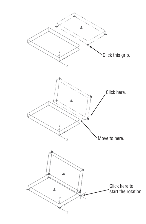
Figure 22-9 The chair after rotating and moving the components
The new UCS orientation enabled you to use the grips to adjust the chair seat and back. All the grip rotation in the previous exercise was confined to the plane of the new UCS. Mirroring and scaling will also occur in relation to the current UCS.
Building 3D Parts in Separate Files
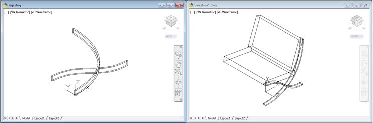
As you work in 3D, your models will become fairly complex. When your model becomes too crowded for you to see things clearly, it helps to build parts of the model and then import them instead of building everything in one file. In the next set of exercises, you’ll draw the legs of the chair and then import them to the main chair file to give you some practice in the procedure.
We’ve prepared a drawing called legs.dwg, which consists of two polylines that describe the shape of the legs. We did this to save you some tedious work that isn’t related to 3D modeling. You’ll use this file as a starting point for the legs, and then you’ll import the legs into the barcelona1.dwg file:
Next you need to change the Thickness property of the two polylines to make them 2″, or 5 cm, wide:
Figure 22-10 The polylines converted to 3D solids
As you’ve just seen, you can convert polylines that have both a width and a thickness into 3D solids. Now you’re ready to add the legs to the rest of the chair:
Figure 22-11 Click and drag the leg from the left window to the right window, and align the leg with the chair seat and back.
In these last few exercises, you worked on the legs of the chair in a separate file and then imported them into the main chair file with a click-and-drag motion. By working on parts in separate files, you can keep your model organized and more manageable. You may have also noticed that, although the legs were drawn in the WCS, they were inserted in the 3DSW UCS that you created earlier. This shows you that imported objects are placed in the current UCS. The same would have happened if you inserted an Xref or another file.
Understanding the UCS Options
You’ve seen how to select a UCS from a set of predefined UCSs. You can frequently use these preset UCSs and make minor adjustments to them to get the exact UCS you want.
You can define a UCS in other ways. You can, for example, use the surface of your chair seat to define the orientation of a UCS. In the following sections, you’ll be shown the various ways you can set up a UCS. Learning how to move effortlessly between UCSs is crucial to mastering the creation of 3D models, so you’ll want to pay special attention to the command options shown in these examples.
Note that these examples are for your reference. You can try them out on your own model. These options are accessible from the View tab’s Coordinates panel.
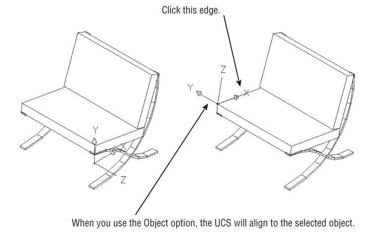
UCS Based on Object Orientation
You can define a UCS based on the orientation of an object. This is helpful when you want to work on a predefined object to fill in details on its surface plane. The following steps are for information only and aren’t part of the tutorial. You can try this at another time when you aren’t working through an exercise.
Follow these steps to define a UCS this way:
Figure 22-12 Using the Object option of the UCS command to locate a UCS
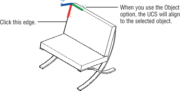
When you create a UCS using the Object option, the location of the UCS origin and its orientation depend on how the selected object was created. Table 22-1 describes how an object can determine the orientation of a UCS.
Table 22-1: Effects of objects on the orientation of a UCS
| Object type | UCS orientation |
| Arc | The center of the arc establishes the UCS origin. The x-axis of the UCS passes through the pick point on the arc. |
| Circle | The center of the circle establishes the UCS origin. The x-axis of the UCS passes through the pick point on the circle. |
| Dimension | The midpoint of the dimension text establishes the UCS origin. The x-axis of the UCS is parallel to the x-axis that was active when the dimension was drawn. |
| Face (of a 3D solid) | The origin of the UCS is placed on a quadrant of a circular surface or on the corner of a polygonal surface. |
| Line | The endpoint nearest the pick point establishes the origin of the UCS, and the XZ plane of the UCS contains the line. |
| Point | The point location establishes the UCS origin. The UCS orientation is arbitrary. |
| 2D polyline | The starting point of the polyline establishes the UCS origin. The x-axis is determined by the direction from the first point to the next vertex. |
| 3D polyline | Returns the message This object does not define a coordinate system. |
| Spline | The UCS is created with its XY plane parallel to the XY plane of the UCS that was current when the spline was created. |
| Solid | The first point of the solid establishes the origin of the UCS. The second point of the solid establishes the x-axis. |
| Trace | The direction of the trace establishes the x-axis of the UCS, and the beginning point sets the origin. |
| 3D Face | The first point of the 3D face establishes the origin. The first and second points establish the x-axis. The plane defined by the 3D face determines the orientation of the UCS. |
| Shapes, text, blocks, attributes, and attribute definitions | The insertion point establishes the origin of the UCS. The object’s rotation angle establishes the x-axis. |
UCS Based on Offset Orientation
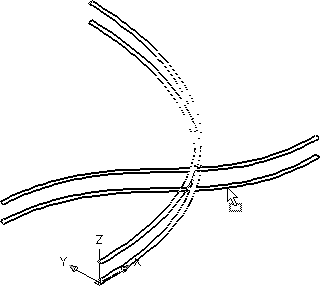
At times, you may want to work in a UCS that has the same orientation as the current UCS but is offset. For example, you might be drawing a building that has several parallel walls offset with a sawtooth effect (see Figure 22-13).
Figure 22-13 Using the Origin option to shift the UCS
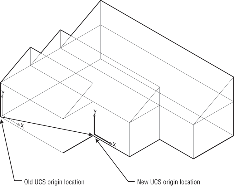
You can easily hop from one UCS to a new, parallel UCS by using the Origin option. Click the Origin tool in the Coordinates panel, or type UCS↵O↵. At the Specify new origin point <0,0,0>: prompt, pick the new origin for your UCS.
Another UCS option, called Move, will move an existing, named UCS to a new location and keep its original orientation. You won’t find the UCS Move option on any panel or toolbar, but you can use it by entering UCS↵M↵ at the Command prompt.
The steps in the following section are for information only and aren’t part of the tutorial. You can try this at another time when you aren’t working through an exercise.
UCS Rotated Around an Axis
Suppose you want to change the orientation of the x-, y-, or z-axis of a UCS. You can do so by using the X, Y, or Z flyout on the View tab’s Coordinates panel. These are perhaps among the most frequently used UCS options:
Figure 22-14 Rotating the UCS about the z-axis
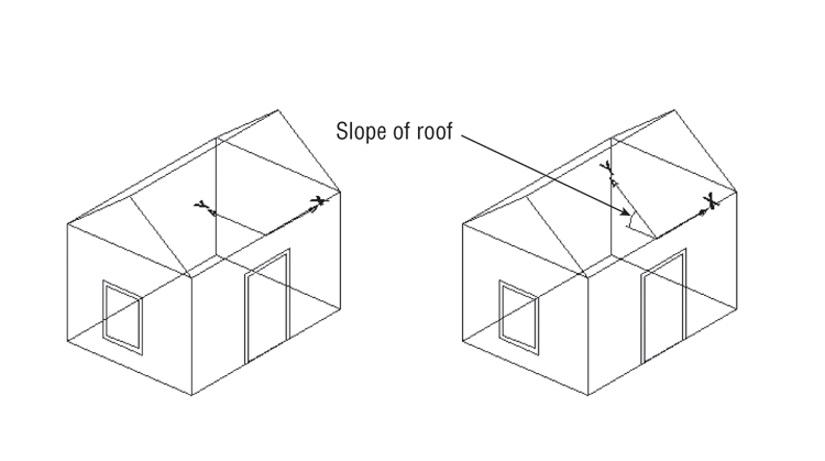
Similarly, the X and Y options enable you to rotate the UCS about the current x- and y-axis, respectively, just as you did for the z-axis earlier. The X and Y tools are helpful in orienting a UCS to an inclined plane. For example, if you want to work on the plane of a sloped roof of a building, you can first use the Origin UCS tool to align the UCS to the edge of a roof and then use the X tool to rotate the UCS to the angle of the roof slope, as shown in Figure 22-15. Note that the default is 90°, so you only have to press ↵ to rotate the UCS 90°, but you can also enter a rotation angle.
Figure 22-15 Moving a UCS to the plane of a sloping roof
Finally, you align the z-axis between two points using the Z-Axis Vector option. This is useful when you have objects in the drawing that you can use to align the z-axis. Here are the steps:
Specify point on positive portion of Z-axis
<0′-0″, 0′-0″, 0′-1″>:Figure 22-16 Picking points for the Z-Axis Vector tool
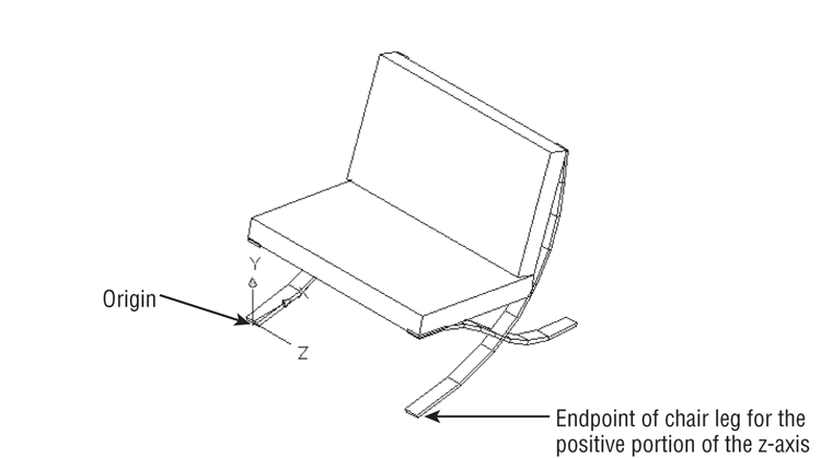
Because your cursor location is in the plane of the current UCS, it’s best to pick a point on an object by using either the Osnap overrides or the coordinate filters.
Orienting a UCS in the View Plane
Finally, you can define a UCS in the current view plane. This points the z-axis toward the user. This approach is useful if you want to switch quickly to the current view plane for editing or for adding text to a 3D view.
Click the View tool in the Coordinates panel, or type UCS↵V↵. Note that the View tool also has a flyout arrowhead that contains the Object and Face tools. If you accidentally click the flyout arrowhead, make sure to click the View tool in the flyout. The UCS icon changes to show that the UCS is aligned with the current view.
AutoCAD uses the current UCS origin point for the origin of the new UCS. By defining a view as a UCS, you can enter text to label your drawing, just as you would in a technical illustration. Text entered in a plane created this way appears normal.
You’ve finished your tour of the UCS command. Set the UCS back to the WCS by clicking the UCS, World tool in the View tab’s Coordinates panel, and save the barcelona1.dwg file.
You’ve explored nearly every option in creating a UCS except one. Later in this chapter, you’ll learn about the 3-Point option for creating a UCS. This is the most versatile method for creating a UCS, but it’s more involved than some of the other UCS options.
Manipulating the UCS Icon
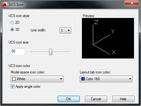
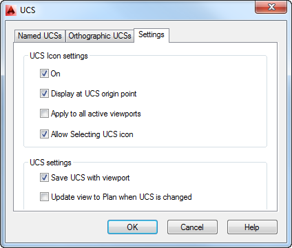
The UCS icon displays the direction of the axes in your drawing file. It can also be directly manipulated by selecting and right-clicking it or by using its multifunction grips. If your UCS icon is not selectable, or to turn off this selectable feature, open the UCS dialog box (click Named in the View tab’s Coordinates panel), click the Settings tab, and see if the Allow Selecting UCS Icon option is checked (see Figure 22-17).
Figure 22-17 Making the UCS icon selectable
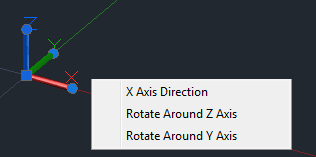
There are essentially two selection options on the icon: the origin and the end of an axis. In either case, select the UCS icon, and then place your cursor over the appropriate grip and click the origin or endpoint (see Figure 22-18). Select how you want to change the UCS (move and align) and move the cursor. The UCS icon will relocate, showing you where your new coordinate system will be. The origin can be moved to a new location or it can be aligned to another object or surface using this method. This makes working in a 3D environment a bit easier. Selecting the origin also allows you to return the current UCS to the World Coordinate System (it resets the UCS). The x-, y-, and z-axes all work the same way. Pick the endpoint of the axis (the grip) to rotate the selected axis about the other axis (for example, if the x-axis is selected, it can rotate about either the y- or z-axis).
Figure 22-18 Selecting and moving the UCS Icon will alter your UCS.
When you right-click the UCS icon, you will see a context menu containing a list of the UCS commands you can choose without having to leave the drawing area. Pick the UCS command you want to access.
Saving a UCS with a View
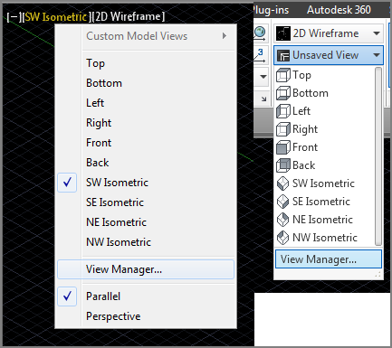
AutoCAD has the ability to save a UCS with a view. Either click the View Manager option in the In-Canvas View Controls (top-left corner of the drawing area) or click the View Manager option, found at the bottom of the 3D Navigation drop-down list in the Home tab’s View panel (see Figure 22-19). In the View Manager dialog box, click the New button. This opens the New View/Shot Properties dialog box. Enter a name for your new view in the View Name box, and then choose a UCS to save with a new view by using the UCS drop-down list in the Settings group of the dialog box. Click OK to complete.
Figure 22-19 Select the View Manager option in either the in-canvas View Controls or the 3D Navigation drop-down list.
Using Viewports to Aid in 3D Drawing
In Chapter 16, “Laying Out Your Printer Output,” you worked extensively with floating viewports in Paper Space. In this section, you’ll use tiled viewports to see your 3D model from several sides at the same time. This is helpful in both creating and editing 3D drawings because it enables you to refer to different portions of the drawing without having to change views.
Tiled viewports are created directly in Model Space, as you’ll see in the following exercise:
Figure 22-20 The Viewports dialog box
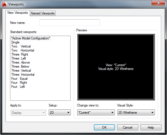
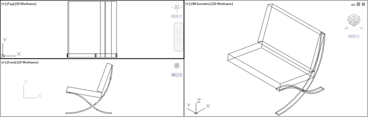
Figure 22-21 Three viewports, each displaying a different view
You’ve set up your viewports. Let’s check to see that your viewport arrangement was saved:
Now, take a close look at your viewport setup. The UCS icon in the orthogonal views in the two left viewports is oriented to the plane of the view. AutoCAD enables you to set up a different UCS for each viewport. The top view uses the WCS because it’s in the same plane as the WCS. The side view has its own UCS, which is parallel to its view. The isometric view to the right retains the current UCS.
A Viewports dialog box option you haven’t tried yet is the Apply To drop-down list in the New Viewports tab (see Figure 22-22).
Figure 22-22 The Apply To drop-down list
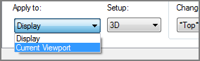
This list shows two options: Display and Current Viewport. When Display is selected, the option you choose from the Standard Viewports list applies to the overall display. When Current Viewport is selected, the option you select applies to the selected viewport in the sample view in the right side of the dialog box. You can use the Current Viewport option to build multiple viewports in custom arrangements.
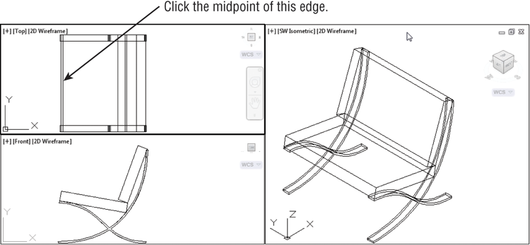
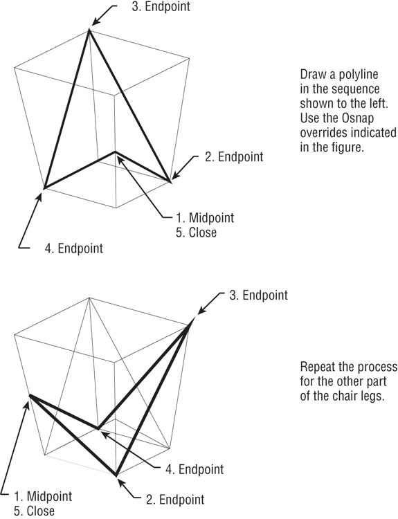
You have the legs for one side. The next step is to mirror those legs for the other side:
Figure 22-23 Mirroring the legs from one side to another
Your chair is complete. Let’s finish by getting a better look at it:
Figure 22-24 Click Single in the Viewport Configurations List drop-down list.
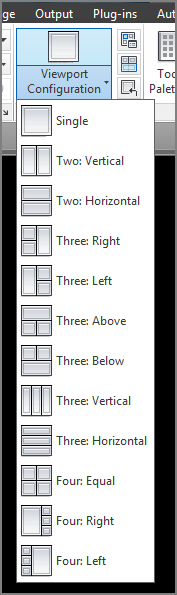
Figure 22-25 The chair in 3D with hidden lines removed
Using the Array Tools
In Chapter 6, “Editing and Reusing Data to Work Efficiently,” you were introduced to the Array command. Let’s take a look at how this works in the 3D world. In AutoCAD 2014, you can create a 3D array from any type of array, whether it is rectangular, polar, or path. Let’s do an example using the path array:
In this exercise, you made an array of a chair that follows the path of an arc. The distance between chairs is 48″ (1219.2 mm), and the vertical riser between each section is 12″ (304.8 mm).
Now suppose you want to adjust the curvature of your array. This is a simple matter of adjusting the shape of the arc, as described in the following exercise:
Here you see how the associative feature of the Arraypath command enables you to control the array by adjusting the object you used for the path. Arrays can be edited through a variety of methods, as you’ll see in the next section.
Making Changes to an Associative Array
Now let’s take a look at how you can make changes to an array. You may have noticed the Associative option in the Array command’s prompt. By default, the Associative option is turned on, which enables you to edit array objects as a group. You’ll see how this works in the following exercises.
You’ll start by editing the array you created using the Path Array tool. You’ll see that the chairs are now skewed and are no longer pointing to the center of the arc. You can realign them by making a simple change to the original chair.
The following steps show you how this is done:
Figure 22-26 The Array tab appears and a new set of panels and options is displayed.

Experiment with other values in the Array tab to see what effects they have.
As you can see from these exercises, you can easily make changes to an array through the Array tab options in the Ribbon. Many of these options are also available through the multifunction grip menus when you have Dynamic Input turned on.
Creating Complex 3D Surfaces
In one of the previous exercises, you drew a chair composed of objects that were mostly straight lines or curves with a thickness. All the forms in that chair were defined in planes perpendicular to one another. For a 3D model such as this, you can get by using the orthographic UCSs. At times, however, you’ll want to draw objects that don’t fit so easily into perpendicular or parallel planes. In the following sections, you’ll create more complex forms by using some of the other 3D commands in AutoCAD.
Laying Out a 3D Form
In this next group of exercises, you’ll draw a butterfly chair. This chair has no perpendicular or parallel planes with which to work, so you’ll start by setting up some points that you’ll use for reference only. This is similar in concept to laying out a 2D drawing. As you progress through the drawing construction, notice how the reference points are established to help create the chair. You’ll also construct some temporary 3D lines to use for reference. These temporary lines will be your layout. These points will define the major UCSs needed to construct the drawing. The main point is to show you some of the options for creating and saving UCSs.
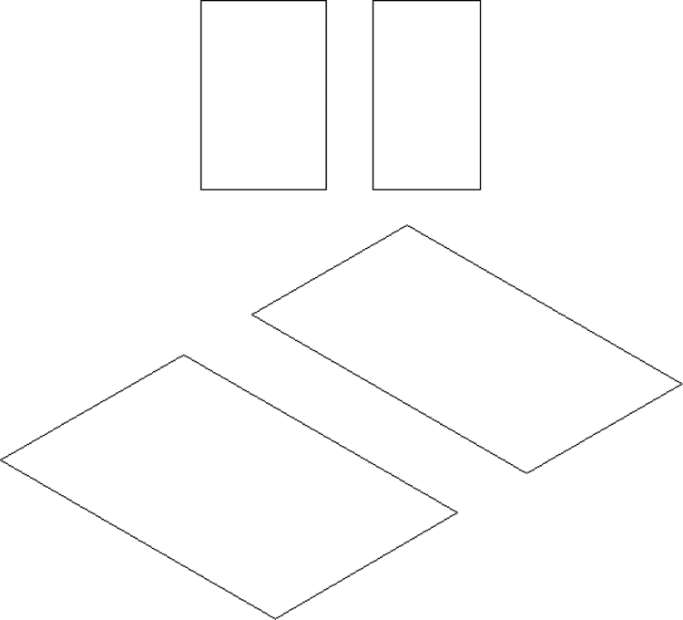
To save time, we’ve created the 2D drawing that you’ll use to build your 3D layout. This drawing consists of two rectangles that are offset by 4″ (10 mm). To make it more interesting, they’re also off-center from each other (see Figure 22-27).
Figure 22-27 Setting up a layout for a butterfly chair
The first thing you’ll need to do is set up the drawing for the layout:
Now you need to move the outer rectangle in the z-axis so its elevation is 30″ (76 cm):
Figure 22-28 The finished chair layout
As an alternate method in step 3, after choosing Move from the Grip Edit context menu, you can turn on Ortho mode and point the cursor vertically so that it shows –Z in the coordinate readout. Then enter 30↵ (76↵ for metric users).
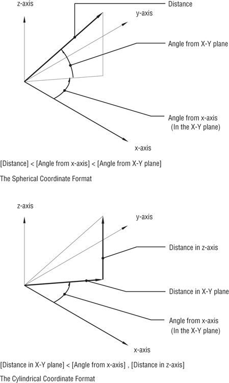
Spherical and Cylindrical Coordinate Formats
In the previous exercise, you used relative Cartesian coordinates to locate the second point for the Move command. For commands that accept 3D input, you can also specify displacements by using the Spherical and Cylindrical Coordinateformats.
The Spherical Coordinate format lets you specify a distance in 3D space while specifying the angle in terms of degrees from the x-axis of the current UCS and degrees from the XY plane of the current UCS (see the top image in Figure 22-29). For example, to specify a distance of 4.5″ (11.43 cm) at a 30° angle from the x-axis and 45° from the XY plane, enter @4.5<30<45 (or @11.43<30<45 for metric users). This refers to the direct distance followed by a < symbol, then the angle from the x-axis of the current UCS followed by another < symbol, and then the angle from the XY plane of the current UCS. To use the Spherical Coordinate format to move the rectangle in the exercise, enter @30<0<90 (or @76<0<90 for metric users) at the Second point: prompt.
The Cylindrical Coordinate format, on the other hand, lets you specify a location in terms of a distance in the plane of the current UCS and a distance in the z-axis. You also specify an angle from the x-axis of the current UCS (see the bottom image in Figure 22-29). For example, to locate a point that is a distance of 4.5″ (11.43 cm) in the plane of the current UCS at an angle of 30° from the x-axis and a distance of 3.3″ (8.38 cm) in the z-axis, enter @4.5<30,3.3 (or @11.43<30,8.38 for metric users). This refers to the distance of the displacement from the plane of the current UCS followed by the < symbol, then the angle from the x-axis followed by a comma, and then the distance in the z-axis. Using the Cylindrical Coordinate format to move the rectangle, you enter @0<0,30 (or @0<0,76 for metric users) at the Second point: prompt.
Figure 22-29 The Spherical and Cylindrical Coordinate formats
Using a 3D Polyline
Now you’ll draw the legs for the butterfly chair by using a 3D polyline. This is a polyline that can be drawn in 3D space. Here are the steps:
Figure 22-30 Using 3D polylines to draw the legs of the butterfly chair
All objects, with the exception of lines and 3D polylines, are restricted to the plane of your current UCS. Two other legacy 3D objects, 3D faces and 3D meshes, are also restricted. You can use the Pline command to draw polylines in only one plane, but you can use the 3DPoly command to create a polyline in three dimensions. 3DPoly objects cannot, however, be given thickness or width.
Creating a Curved 3D Surface
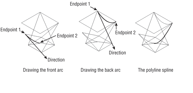
Next, you’ll draw the seat of the chair. The seat of a butterfly chair is usually made of canvas, and it drapes from the four corners of the chair legs. You’ll first define the perimeter of the seat by using arcs, and then you’ll use the Edge Surface tool in the Home tab’s Modeling panel to form the shape of the draped canvas. The Edge Surface tool creates a surface based on four objects defining the edges of that surface. In this example, you’ll use arcs to define the edges of the seat.
To draw the arcs defining the seat edges, you must first establish the UCSs in the planes of those edges. In the previous example, you created a UCS for the side of the chair before you could draw the legs. In the same way, you must create a UCS defining the planes that contain the edges of the seat.
Because the UCS you want to define isn’t orthogonal, you’ll need to use the 3-point method. This lets you define the plane of the UCS based on three points:
Figure 22-31 Defining and saving three UCSs
You’ve defined and saved a UCS for the front side of the chair. As you can see from the UCS icon, this UCS is at a nonorthogonal angle to the WCS. Continue by creating UCSs for two more sides of the butterfly chair:
Figure 22-32 Drawing the front and back seat edge using arcs and a polyline spline
Next you’ll mirror the side-edge spline to the opposite side. This will save you from having to define a UCS for that side:
Figure 22-33 Set your UCS to World, and then mirror the arc that defines the side of the chair seat.
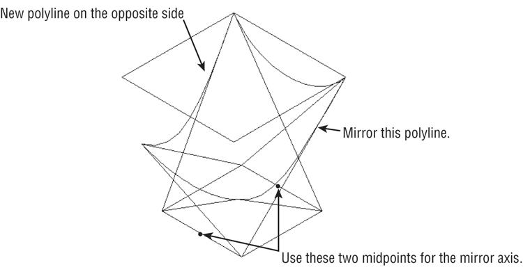
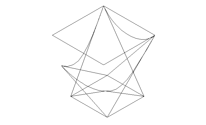
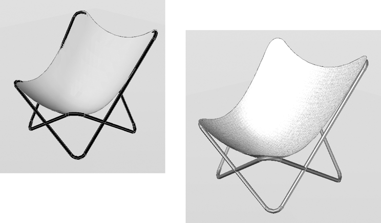
Figure 22-34 Your butterfly chair so far.
Finally, let’s finish this chair by adding the mesh representing the chair seat:
Figure 22-35 The butterfly chair with a mesh seat
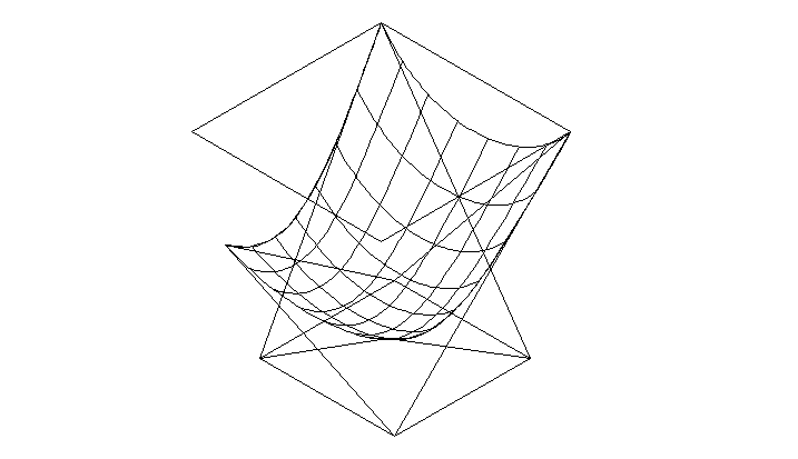
You’ve got the beginnings of a butterfly chair with the legs drawn in schematically and the seat as a 3D surface. You can add some detail by using a few other tools, as you’ll see in the next set of exercises.
Converting the Surface into a Solid
In the previous example, you used the Loft tool to create a 3D surface. Once you have a surface, you can convert it to a solid to perform other modifications.
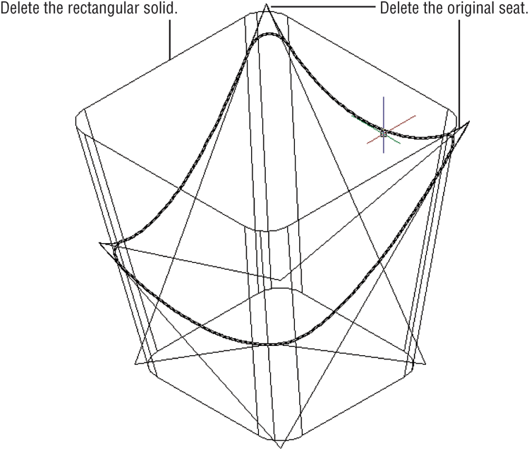
You’ll want to round the corners of the seat surface to simulate the way a butterfly chair hangs off its frame. You’ll also round the corners of the frame and turn the frame into a tubular form. Start by rounding the seat surface. This will involve turning the surface into a solid so that you can use solid-editing tools to get the shape you want:
The seat surface appears to lose its webbing, but it has just been converted to a very thin 3D solid.
Shaping the Solid
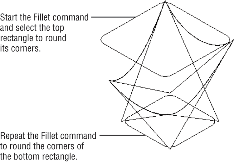
The butterfly chair is in a fairly schematic state. The corners of the chair are sharply pointed, whereas a real butterfly chair would have rounded corners. In this section, you’ll round the corners of the seat with a little help from the original rectangles you used to form the layout frame.
First you’ll use the Fillet command to round the corners of the rectangles. Then you’ll use the rounded rectangles to create a solid from which you’ll form a new seat:
Figure 22-36 Round the corners of the rectangles with the Fillet command.
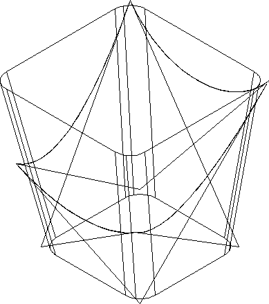
Next create a 3D solid from the two rectangles using the Loft tool:
Figure 22-37 The lofted rectangles form a 3D solid.
Finding the Interference Between Two Solids
In this next exercise, you’ll use a tool that is intended to find the interference between two solids. This is useful if you’re working with crowded 3D models and you need to check whether objects may be interfering with each other. For example, a mechanical designer might want to check to make sure duct locations aren’t passing through a structural beam.
You’ll use Interfere as a modeling tool to obtain a shape that is a combination of two solids: the seat and the rectangular solid you just created. Here are the steps:
Figure 22-38 Checking for interference
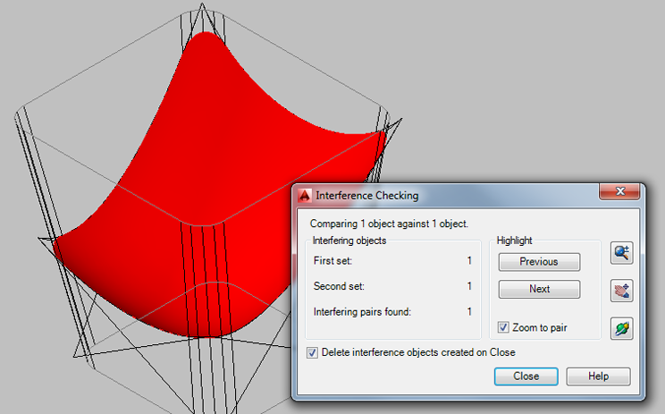
Figure 22-39 The interference solid appears on top of the original seat.
As mentioned earlier, the Interference Checking tool is intended to help you find out whether objects are colliding in a 3D model; as you’ve just seen, though, it can be an excellent modeling tool that can help you derive a form that you may not otherwise have the ability to create.
A number of other options are available when you’re using the Interference Checking tool. Table 22-2 lists the options in the Interference Checking dialog box.
Table 22-2: Interference Checking dialog box options
| Option | What it does |
| First Set | Specifies the number of objects in the first set of selected objects |
| Second Set | Specifies the number of objects in the second set of selected objects |
| Interfering Pairs Found | Indicates the number of interferences found |
| Previous | Highlights the previous interference object |
| Next | Highlights the next interference object if multiple objects are present |
| Zoom To Pair | Zooms to the interference object while you’re using the Previous and Next options |
| Zoom Realtime | Closes the dialog box to allow you to use Zoom Realtime |
| Pan Realtime | Closes the dialog box to allow you to use Pan |
| 3D Orbit | Closes the dialog box to allow you to use 3D Orbit |
| Delete Interference Objects Created On Close | Deletes the interference object after the dialog box is closed |
The prompt for the Interference Checking command also showed some options. The prompt in step 2 shows Nested selection/Settings. The Nested selection option lets you select objects that are nested in a block or an Xref. The Settings option opens the Interference Settings dialog box (see Figure 22-40).
Figure 22-40 Settings for interference
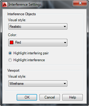
This dialog box offers settings for the temporary display of interference objects while you’re using the Interference command. Table 22-3 lists the options for this dialog box.
Table 22-3: Interference Settings dialog box options
| Option | What it does |
| Visual Style | Controls the visual style for interference objects |
| Color | Controls the color for interference objects |
| Highlight Interfering Pair | Highlights the interfering objects |
| Highlight Interference | Highlights the resulting interference objects |
| Visual Style | Controls the visual style for the drawing while displaying the interference objects |
Creating Tubes with the Sweep Tool
You need to take care of one more element before your chair is complete. The legs are currently simple lines with sharp corners. In this section, you’ll learn how you can convert lines into 3D tubes. To make it more interesting, you’ll add rounded corners to the legs.
Start by rounding the corners on the lines you’ve created for the legs:
Figure 22-41 Drawing the circles for the tubes
The chair is almost complete, but the legs are just wireframes. Next you’ll give them some thickness by turning them into tubes. Start by creating a set of circles. You’ll use the circles to define the diameter of the tubes:
Now you’re ready to form the tubes:
Figure 22-42 A perspective view of the butterfly chair with tubes for legs
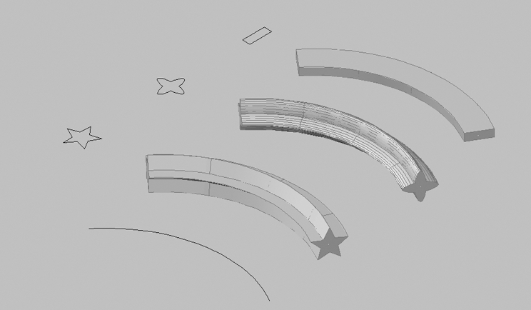
Using Sweep to Create Complex Forms
Although you used circles with the Sweep command to create tubes, you can use any closed polyline shape. Figure 22-43 gives some examples of other shapes you can use with the Sweep command.
Figure 22-43 You can use any closed shape with the Sweep command.
In step 3 of the previous exercise, you may have noticed some command-line options. These options offer additional control over the way Sweep works. Here is a rundown on how they work:
Figure 22-44 Alignment lets you set the angle between the object to sweep and the sweep path.
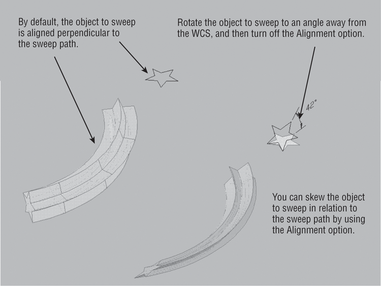
Figure 22-45 Using the Base Point option
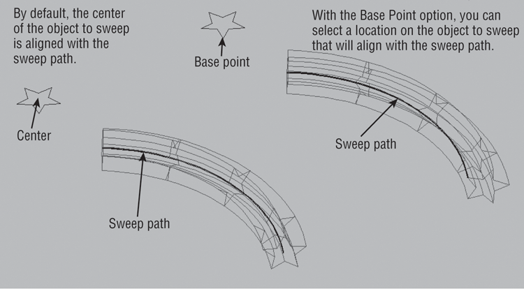
Figure 22-46 Scale lets you scale the object to sweep as it’s swept along the path.
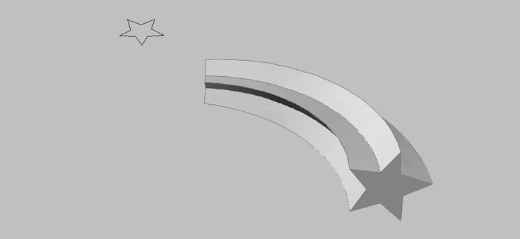
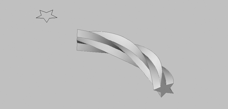
Figure 22-47 You can have the object sweep twist along the path to create a spiral effect.
These options are available as soon as you select the sweep object and before you select the path object. You can use any combination of options you need. For example, you can apply the Twist and Scale options together, as shown in Figure 22-48.
Figure 22-48 The Scale and Twist options applied together
Creating Spiral Forms
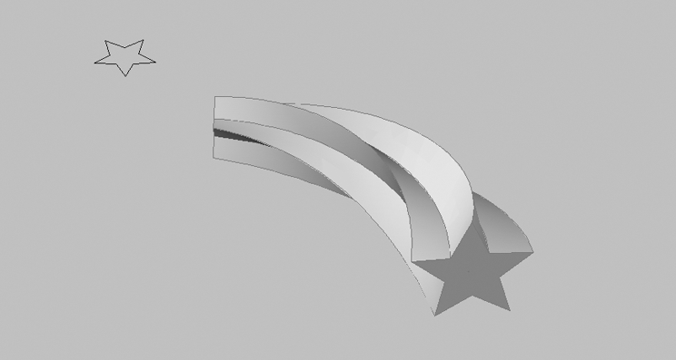
You can use the Sweep tool in conjunction with the Helix tool to create a spiral form, such as a spring or the threads of a screw. You’ve already seen how the Sweep tool works. Try the following to learn how the Helix tool works firsthand.
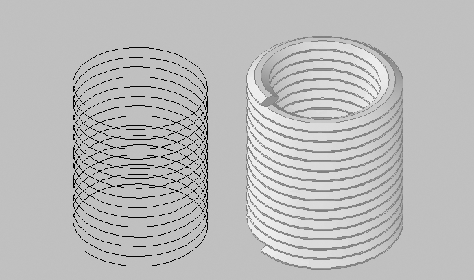
In this exercise, you’ll draw a helicoil thread insert. This is a device used to repair stripped threads; it’s basically a coiled steel strip that forms internal and external threads. Here are the steps:
Number of turns = 3.0000  Twist=CCW
Specify center point of base:Figure 22-49 The helix and the helicoil after using Sweep
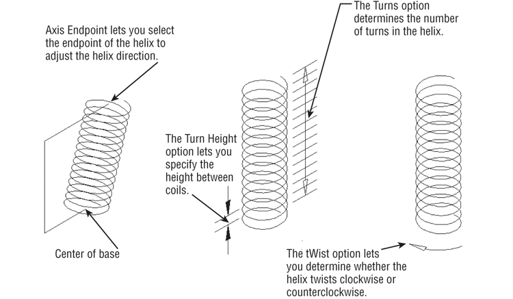
In step 6, you used the Turns option to specify the total number of turns in the helix. You also have other options that give you control over the shape of the helix. Figure 22-50 shows you the effects of the Helix command options. You may want to experiment with them on your own to become familiar with Helix.
Figure 22-50 The Helix command options
Now use the Sweep tool to complete the helicoil:
If the space between the coils is too small for the cross section, you may get an error message. If you get an error message at step 3, make sure you created the helix exactly as specified in the previous exercise. You may also try increasing the helix height.
In step 3, instead of selecting the sweep path, you can select an option to apply to the object to sweep. For example, by default, Sweep aligns the object to sweep at an angle that is perpendicular to the path and centers it. See “Using Sweep to Create Complex Forms” earlier in this chapter.
Creating Surface Models
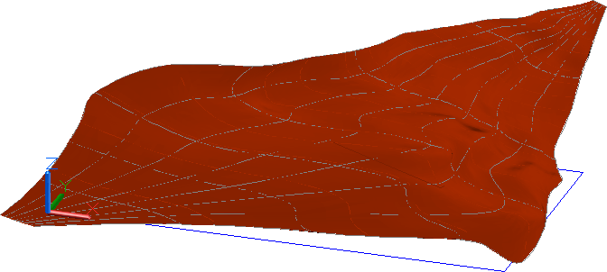
In an earlier exercise, you used the Loft command to create the seat of a butterfly chair. In this section, you’ll return to the Loft command to explore some of its other uses. This time, you’ll use it to create a 3D model of a hillside based on a set of site-contour lines. You’ll also see how you can use a surface created from the Loft command to slice a solid into two pieces, imprinting the solid with the surface shape.
Start by creating a 3D surface using the Loft command:
Figure 22-51 Creating a 3D surface from contour lines
Once the loft surface has been placed, you can make adjustments to the way the loft is generated by using the arrow grip that appears when you select the surface:
Figure 22-52 The surface showing the multifunction grip menu with the Ruled option selected
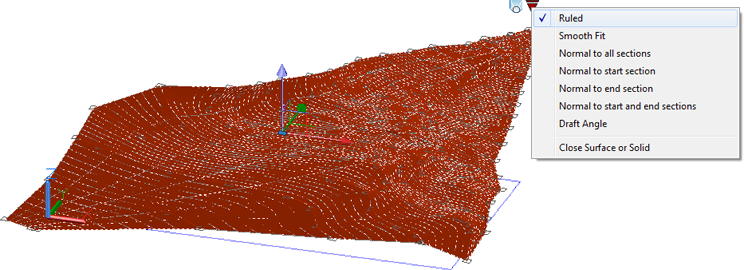
In the butterfly chair exercise, you used the Guides option in the Loft Command prompt. This allowed you to use the polyline curves to guide the loft shape from the front arc to the back arc. In this exercise, you didn’t use the command options and went straight to the multifunction grip menu. The Ruled setting that you used in step 3 generates a surface that connects the cross sections in a straight line.
Slicing a Solid with a Surface
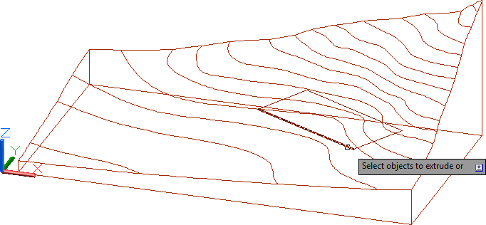
In the barcelona1.dwg chair example, you converted a surface into a solid using the Thicken command. Next, you’ll use a surface to create a solid in a slightly different way. This time, you’ll use the surface to slice a solid into two pieces. This will give you a form that is more easily read and understood as a terrain model:
Figure 22-53 The box extruded through the contours
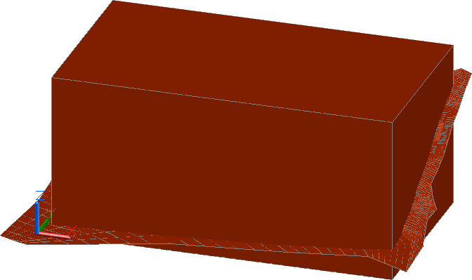
You may have noticed that, as you raised the box height, you could see how it intersected the contour surface. Next you’ll slice the box into two pieces:
Figure 22-54 The box with the contour surface imprinted
In step 3, you saw a prompt that offered a variety of methods for slicing the box. The Surface option allowed you to slice the box using an irregular shape, but most of the other options let you slice a solid by defining a plane or a series of planar objects.
Finding the Volume of a Cut
Civil engineers frequently ask us how they can find the volume of earth from an excavated area. This is often referred to as a cut from a cut and fill operation. To do this, you first have to create the cut shape. Next you use the Interfere command to find the intersection between the cut shape and the contour surface. You can then find the volume of the cut shape using one of the inquiry commands in AutoCAD. The following exercise demonstrates how this is done.
Suppose that the contour model you’ve just created represents a site where you’ll excavate a rectangular area for a structure. You want to find the amount of earth involved in the excavation. A rectangle has been placed in the contour drawing representing such an area:
Figure 22-55 Select Wireframe from the Visual Styles flyout.
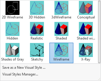
Figure 22-56 Selecting the rectangle representing the excavation area
Here you used the Selection Cycling tool to help you select the rectangle, which is overlapped by the contour solid. The Selection Cycling tool presents the Selection dialog box, which lets you determine the type of object you want to select, thereby filtering out other objects nearby that might be selected accidentally.
With the excavation rectangle in place, you can use the Interfere command to find the volume of the excavation:
Figure 22-57 The 3D solid representing the excavation
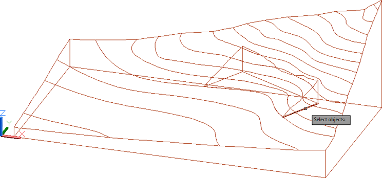
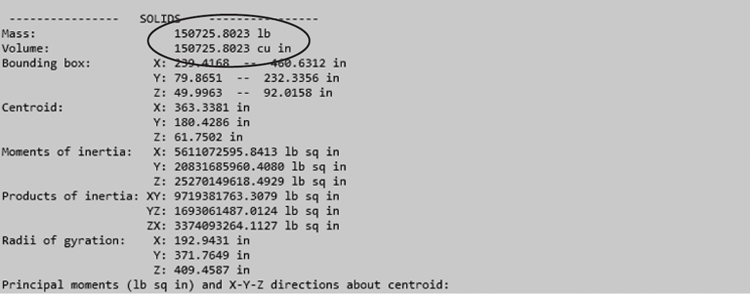
Figure 22-58 The mass and volume information from the Region/Mass Properties tool
Understanding the Loft Command
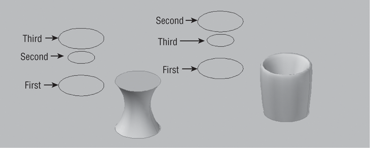
As you’ve seen from the exercises in this chapter, the Loft command lets you create just about any shape you can imagine, from a simple sling to the complex curves of a contour map. If your loft cross sections are a set of closed objects like circles or closed polygons, the resulting object is a 3D solid instead of a surface.
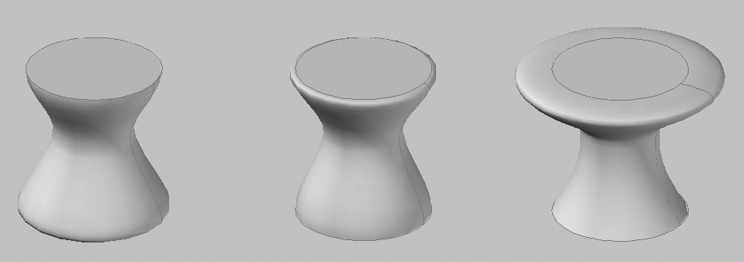
The order in which you select the cross sections is important because Loft will follow your selection order to create the surface or solid. For example, Figure 22-59 shows a series of circles used for a lofted solid. The circles on each side are identical in size and placement, but the order of selection is different. The solid on the left was created by selecting the circles in consecutive order from bottom to top, creating an hourglass shape. The solid on the right was created by selecting the two larger circles first from bottom to top; the smaller, intermediate circle was selected last. This selection order created a hollowed-out shape with more vertical sides.
Figure 22-59 The order in which you select the cross sections affects the result of the Loft command.
In addition to the selection order, several other settings affect the shape of a solid created by the Loft command. In the contour-map example, you selected the Ruled setting from a multifunction grip after you had completed the Loft command. You can also set Loft command options through the Loft Settings dialog box (see Figure 22-60). This dialog box appears during the Loft command when you select the Settings option after you’ve selected a set of cross sections.
Figure 22-60 Loft Settings Smooth Fit
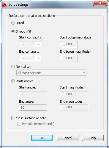
You can radically affect the way the Loft command forms a surface or a solid through the options in this dialog box, so it pays to understand what those settings do. Take a moment to study the following sections that describe the Loft Settings dialog box options.
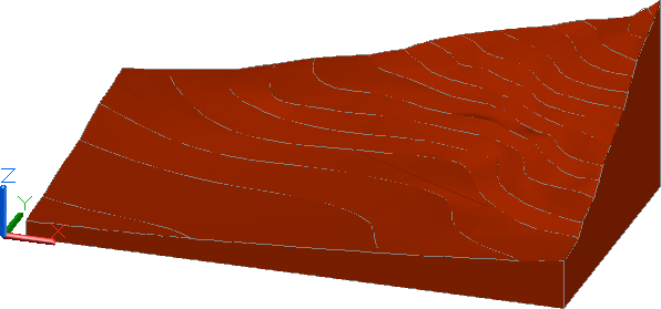
Ruled and Smooth Fit
The Ruled option connects the cross sections with straight surfaces, as shown in the sample to the left in Figure 22-61.
Figure 22-61 Samples of a Ruled loft at left and a Smooth Fit loft on the right
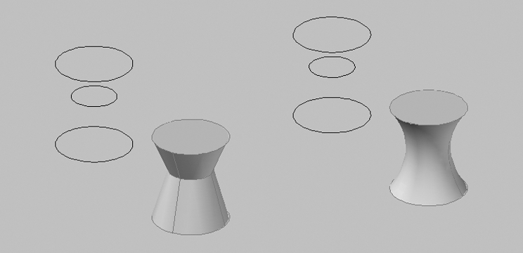
The Smooth Fit option connects the cross sections with a smooth surface. It attempts to make the best smooth transitions between the cross sections, as shown in the right image in Figure 22-61.
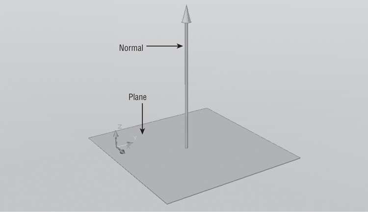
Normal To
Normal To is a set of four options presented in a drop-down list. To understand what this setting does, you need to know that normal is a mathematical term referring to a direction that is perpendicular to a plane, as shown in Figure 22-62. In these options, normal refers to the direction the surface takes as it emerges from a cross section.
Figure 22-62 A normal is a direction perpendicular to a plane.
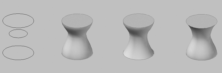
If you use the All Cross Sections option, the surfaces emerge in a perpendicular direction from all the cross sections, as shown in the first image in Figure 22-63. If you use the End Cross Section option, the surface emerges in a direction that is perpendicular to just the end cross section, as shown in the second image in Figure 22-63. The Start Cross Section option causes the surface to emerge in a direction perpendicular to the start cross section. The Start And End Cross Sections option combines the effect of the Start Cross Section and End Cross Section options.
Figure 22-63 Samples of the Normal To options applied to the same set of cross sections
Draft Angles
The Draft Angles option affects only the first and last cross sections. This option generates a smooth surface with added control over the start and end angles. Unlike the Normal To option, which forces a perpendicular direction to the cross sections, Draft Angles allows you to set an angle for the surface direction. For example, if you set Start Angle to a value of 0, the surface will bulge outward from the start cross section, as shown in the first image of Figure 22-64.
Figure 22-64 The Draft Angles options
Likewise, an End Angle setting of 0 will cause the surface to bulge at the end cross section (see the second image in Figure 22-64).
The Start and End Magnitude settings let you determine a relative strength of the bulge. The right image in Figure 22-64 shows a draft angle of 0 and magnitude of 50 for the last cross section.
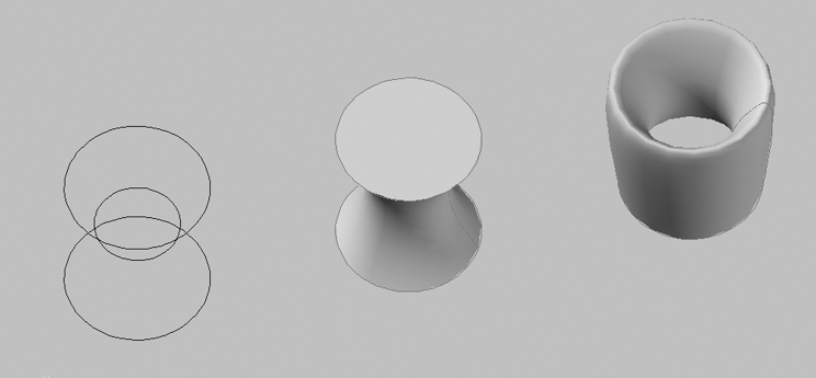
Close Surface or Solid
The Close Surface Or Solid option is available only when the Smooth Fit option is selected. It causes the first and last cross section objects to be connected, so the surface or solid loops back from the last to the first cross section. Figure 22-65 shows the cross sections at the left, a smooth version in the middle, and a smooth version with the Close Surface Or Solid option turned on. The Close Surface Or Solid option causes the solid to become a tube.
Figure 22-65 The Close Surface Or Solid option connects the end and the beginning cross sections.
Moving Objects in 3D Space
AutoCAD provides three tools specifically designed for moving objects in 3D space: 3D Align, 3D Move, and 3D Rotate. You can find all three commands in the Home tab’s Modify panel. These tools help you perform common moves associated with 3D editing.
Aligning Objects in 3D Space
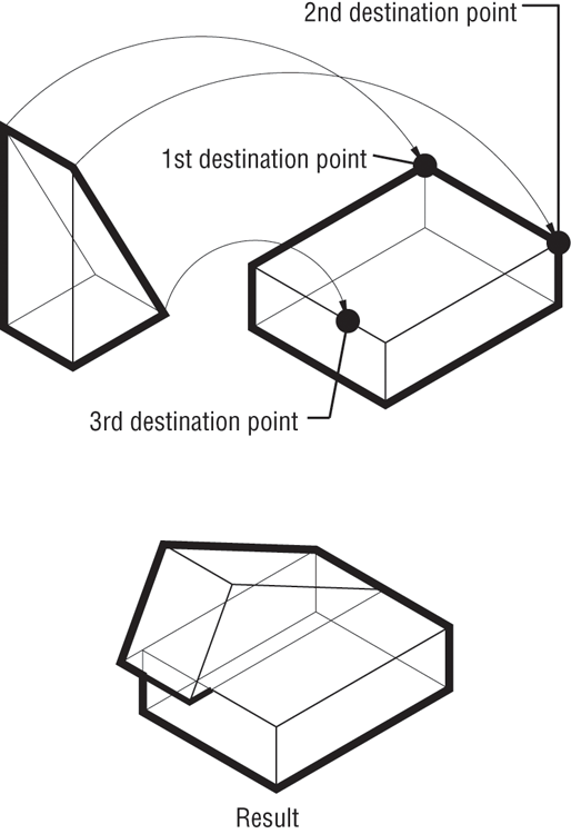
In mechanical drawing, you often create the parts in 3D and then show an assembly of the parts. The 3D Align command can greatly simplify the assembly process. The following steps show how to use 3D Align to line up two objects at specific points:
Figure 22-66 Aligning two 3D objects
Moving an Object in 3D
In Chapter 21, you saw how you can use the move gizmo tool to help restrain the motion of an object in the x-, y-, or z-axis. AutoCAD offers a Move command specifically designed for 3D editing that includes a move gizmo tool to restrain motion.
You don’t need to perform these steps as an exercise. You can try the command on your own when you need to use it.
Here’s how it works:
Figure 22-67 The Move gizmo
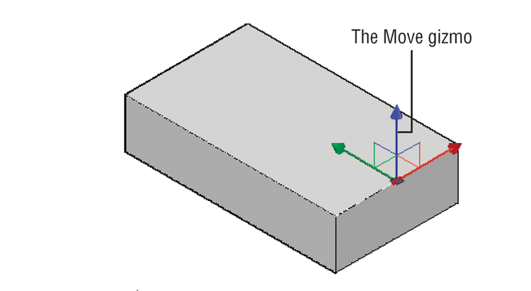
Figure 22-68 An axis vector appears when you hover over an axis of the gizmo.
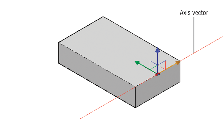
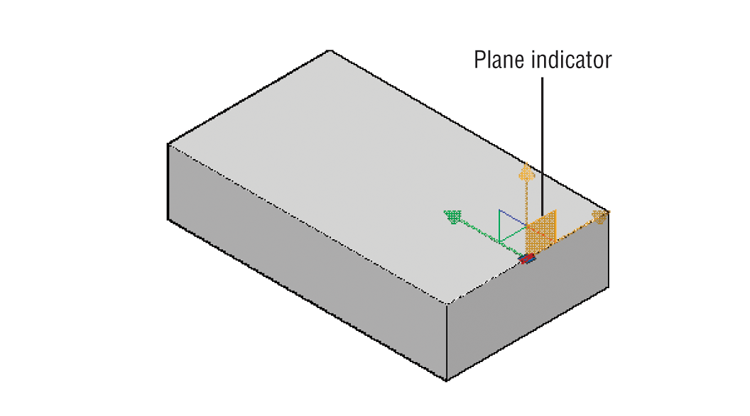
Alternately, in step 3, you can hover over and click a plane indicator on the gizmo to restrain the motion along one of the planes defined by two of the axes (see Figure 22-69).
Figure 22-69 Hover over the plane indicator to restrain the motion along a plane.
Rotating an Object in 3D
The 3D Rotate command is another command that is like an extension of its 2D counterpart. With 3D Rotate, a Rotate gizmo appears that restrains the rotation about the x-, y-, or z-axis.
You don’t need to perform these steps as an exercise. You can try the command on your own when you need to use it.
Here’s how it works:
Figure 22-70 The Rotate gizmo
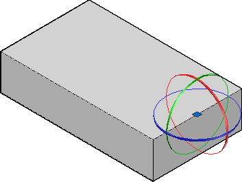
You can also just select one of the circles in step 3 instead of selecting a base point. If you do this, then the selected object begins to rotate. You don’t have to select a start and end angle.