CHAPTER
5

Data Science Craftsmanship, Part II

In the previous chapter, you discovered a number of data science techniques and recipes, including visualizing data with data videos, new types of metrics, computer science topics, and questions to ask when choosing a vendor, as well as a comparison between data scientists, statisticians, and data engineers.

In this chapter, you consider material that is less focused on metrics and more focused on applications. It includes discussions on how to create a data dictionary, hidden decision trees, hash joins in the context of NoSQL databases, and the first Analyticbridge Theorem, which provides a simple, model-free, nonparametric way to compute confidence intervals without statistical theory or knowledge.

This chapter is less statistical theory–oriented compared with the previous chapter. The topics discussed in this chapter are typically classified as data analyses rather than statistical or computer analyses. Most of the material has not been published before. Case studies, applications, and success stories are discussed in the next chapter.

The topics discussed in this chapter, such as hidden decision trees, data dictionaries, and hash joins, are important subjects for data scientists because they are at the intersection of statistics and computer science, and are designed to handle big data. Traditional statisticians typically don't learn or use these techniques, but data scientists do.

Data Dictionary

One of the most valuable tools when performing exploratory analyses is building a data dictionary, which offers the following advantages:

• Identify areas of sparseness and areas of concentration in high-dimensional data sets.
• Identify outliers and data glitches.
• Get a good sense of what the data contains and where to spend time (or not) in further data mining.

What Is a Data Dictionary?

A data dictionary is a table with three or four columns. The first column represents a label, that is, the name of a variable or a combination of multiple (up to three) variables. The second column is the value attached to the label: the first and second columns actually constitute a name-value pair. The third column is a frequency count: it measures how many times the value (attached to the label in question) appears in the data set. You can add a fourth column to specify the dimension of the label (1 if it represents one variable, 2 if it represents a pair of variables, and so on).

Typically, you include all labels of dimension 1 and 2 with count > threshold (for example, threshold = 5), but no or only few values (the ones with high count) for labels of dimension 3. Labels of dimension 3 should be explored after having built the dictionary for dim 1 and 2, by drilling down on name-value pair of dim 2 that have a high count.

An example of a data dictionary entry is category∼keyword travel∼Tokyo 756 2. In this example, the entry corresponds to a label of dimension 2 (as indicated in column 4), and the simultaneous combination of the two values (travel, Tokyo) is found 756 times in the data set.

The first thing you want to do with a dictionary is to sort it using the following 3-dim index: column 4, then column 1, and then column 3. Then look at the data and find patterns.

Building a Data Science Dictionary

Browse your data set sequentially. For each observation, store all name-value pair of dim 1 and dim 2 as hash table keys, and increment count by 1 for each of these labels/values. In Perl, it can be performed with code such as $hash{“$label $value”}++.

If the hash table grows large, stop, save the hash table on file, and then delete it in memory and resume where you paused, with a new hash table. At the end, merge hash tables after ignoring hash entries where count is too small.

Hidden Decision Trees

Hidden decision trees (HDT) is a technique created and patented by me (see http://bit.ly/1h9mXZr) to score large volumes of transaction data. It blends robust logistic regression with hundreds of small decision trees (each one representing, for instance, a specific type of fraudulent transaction) and offers significant advantages over both logistic regression and decision trees: robustness, ease of interpretation, no tree pruning. and no node splitting criteria. It makes this methodology powerful and easy to implement, even for someone with no statistical background.

HDT is a statistical and data mining methodology (just like logistic regression, SVM, neural networks, or decision trees) to handle problems with large amounts of data, nonlinearity, and strongly correlated dependent variables. I developed it after discovering how sparse (or noisy) big data usually is, with valuable information (signal) concentrated in just tiny pieces of the data sets—just like stars and matter represent a very tiny fraction of the universe. HDT removes the complexity, instability, arbitrary parameters, and lack of interpretation found in traditional large decision trees. It also eliminates the failure of traditional logistic regressions to identify highly nonlinear structures by blending regression with some sort of decision tree. HDT was first applied in the context of optimum features selection to score credit card transactions to detect fraud. The technique is easy to implement in any programming language. It is more robust than decision trees or logistic regression and helps detect natural final nodes. Implementations typically rely heavily on large, granular hash tables.

No decision tree is actually built (thus the name hidden decision trees), but the final output of a hidden decision tree procedure consists of a few hundred nodes from multiple non-overlapping small decision trees. Each of these parent (invisible) decision trees corresponds, for example, to a particular type of fraud in fraud detection models. Interpretation is straightforward, in contrast with traditional decision trees.

The methodology was first invented in 2003 in the context of credit card fraud detection. It is not implemented in any statistical package at this time. Hidden decision trees are frequently combined with logistic regression in a hybrid scoring algorithm, where 80 percent of the transactions are scored via hidden decision trees, while the remaining 20 percent are scored using a compatible logistic regression type of scoring.

Hidden decision trees take advantage of the structure of large multivariate features typically observed when scoring a large number of transactions, for example, for fraud detection. The technique is not connected with hidden Markov fields.

Potential applications of HDT include the following:

• Fraud and spam detection
• Web analytics
  • Keyword scoring/bidding (ad networks and paid search)
  • Transaction scoring (click, impression, conversion, and action)
  • Click fraud detection
  • Website scoring, ad scoring, landing page or advertiser scoring
  • Collective filtering (social network analytics)
  • Relevancy algorithms
• Text mining
  • Scoring and ranking algorithms
  • Infringement and spam detection
  • Sentiment analysis

The way HDT is applied to these problems is as follows: in a typical machine learning approach, rule sets or association rules are used to solve these problems. For instance, if an e-mail message contains the keyword “breast” or other keyword from a keyword blacklist, but not “breast cancer,” which is white-listed, then it increases the spam score. If many rules get triggered, the spam score is very high. HDT automatically sets weights to these various rules and automatically detects, among millions (or billions) of rules, which ones should be kept and combined.

Since first developing HDT, I have further refined the model over the past 10 years, as follows:

• 2003: First version applied to credit card fraud detection
• 2006: Application to click scoring and click fraud detection
• 2008: More advanced versions to handle granular and large data sets, such as:
  • Hidden forests: Multiple HDTs, each one applied to a cluster of correlated rules
  • Hierarchical HDTs: The top structure, not just rule clusters, is modeled using HDTs.
  • Non-binary rules: Naïve Bayes blended with HDTs.

Implementation

The model presented here is used in the context of click scoring. The purpose is to create predictive scores, where score = f(response), that is, score is a function of the response. The response is sometimes referred to as the dependent variable in statistical and predictive models. Examples of responses include:

• Odds of converting (Internet traffic data — hard or soft conversions)
• CR (conversion rate)
• Probability that transaction is fraudulent

Independent variables are called features or rules. They are highly correlated.

Traditional models to be compared with HDTs include logistic regression, decision trees, and naïve Bayes.

HDTs use a one-to-one mapping between scores and multivariate features. A multivariate feature is a rule combination attached to a particular transaction (that is, a vector specifying which rules are triggered and which ones are not) and is sometimes referred to as a flag vector or node.

HDT fundamentals based on a typical data set are:

• If you use 40 binary rules, you have 2 at power 40 potential multivariate features.
• If a training set has 10 MM transactions, you will obviously observe 10 MM multivariate features at most, a number much smaller than 2 at power 40.
• 500 out of 10 MM features account for 80 percent of all transactions.
• The top 500 multivariate features have a strong predictive power.
• An alternative algorithm is required to classify the remaining 20 percent of transactions.
• Using neighboring top multivariate features to score the remaining 20 percent of transactions creates bias, as rare multivariate features (sometimes not found in the training set) correspond to observations that are worse than average, with a low score (because they trigger many fraud detection rules).

Implementation Details

Each top node (or multivariate feature) is a final node from a hidden decision tree. There is no need for tree pruning or splitting algorithms and criteria: HDT is straightforward and fast, and can rely on efficient hash tables (where key = feature and value = score). The top 500 nodes, used to classify (that is, score) 80 percent of transactions, come from multiple hidden decision trees—hidden because you never used a decision tree algorithm to produce them.

The remaining 20 percent of transactions are scored using an alternative methodology (typically, logistic regression). Thus HDT is a hybrid algorithm, blending multiple, small, easy-to-interpret, invisible decision trees (final nodes only) with logistic regression.

Note that in the logistic regression, you can use constrained regression coefficients. These coefficients depend on two or three top parameters and have the same sign as the correlation between the rule they represent and the response or score. This makes the regression non-sensitive to high cross correlations among the “independent” variables (rules), which are indeed not independent in this case. This approach is similar to ridge regression, logic regression, or Lasso regression. The regression is used to fine-tune the top parameters associated with regression coefficients. Approximate solutions (you are doing approximate logistic regression here) are—if well designed—almost as accurate as exact solutions but can be far more robust.

You deal with these types of scores:

• The top 500 nodes provide a score S₁ available for 80 percent of the transactions.
• The logistic regression provides a score S₂ available for 100 percent of the transactions.

To blend the scores, you would do the following:

• Rescale S₂ using the 80 percent transactions that have two scores, S₁ and S₂. Rescaling means applying a linear transformation so that both scores have the same mean and the same variance. Let S₃ be the rescaled S₂.
• Transactions that can't be scored with S₁ are scored with S₃.

HDT nodes provide an alternative segmentation of the data. One large, mediumscore segment corresponds to neutral transactions (triggering no rule). Segments with low scores correspond to specific fraud cases. Within each segment, all transactions have the same score. HDT provide a different type of segmentation than principal component analysis (PCA) and other analyses.

Example: Scoring Internet Traffic

Figure 5-1 shows the score distribution with a system based on 20 rules, each one having a low triggering frequency. It has the following features:

• Reverse bell curve
• Scores below 425 correspond to unbillable transactions.
• Spikes at the bottom and top of the score scale
• 50 percent of all transactions have good scores.
• Scorecard parameters
  • A drop of 50 points represents a 50 percent drop in the conversion rate.
  • The average score is 650.
• Model improvement: from reverse bell curve to bell curve
  • Transaction quality versus fraud detection
  • Add antirules, perform score smoothing (also removes score caking)

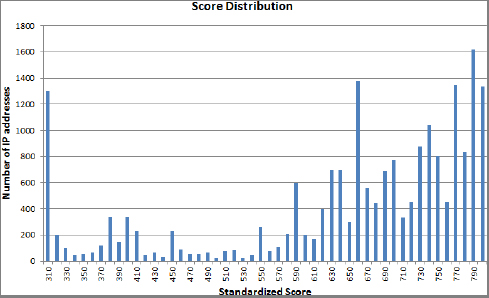
Figure 5-2 shows a comparison of scores with conversion rates (CR). HDTs were applied to Internet data, scoring clicks with a score used to predict chances of conversion (a conversion being a purchase, a click out, or a sign-up on some landing page). Overall, you have a rather good fit.

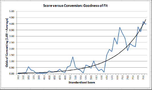
Peaks in the figure could mean:

• Bogus conversions (happens a lot if conversion is simply a click out)
• Residual noise
• Model needs improvement (incorporate antirules)

Valleys could mean:

• Undetected conversions (cookie issue, time-to-conversion unusually high)
• Residual noise
• Model needs improvement

Conclusion

HDT is a fast algorithm, easy to implement, and can handle large data sets efficiently, and the output is easy to interpret. It is nonparametric and robust. The risk of over-fitting is small if no more than the top 500 nodes are selected and ad hoc cross-validation techniques are used to remove unstable nodes. It offers a built-in, simple mechanism to compute confidence intervals for scores (see the next section).

HDT is an algorithm that can detect multiple types of structures: linear structures via the regression and nonlinear structures via the top nodes. Future directions for HDT could include hidden forests to handle granular data and hierarchical HDTs.

Model-Free Confidence Intervals

Here you can find easy-to-compute, distribution-free, fractional confidence intervals. If observations from a specific experiment (for instance, scores computed on 10 million credit card transactions) are assigned a random bin ID (labeled 1, ···, N) then you can easily build a confidence interval for any proportion or score computed on these k random bins, using the Analyticbridge Theorem described next.

Methodology

Say you want to estimate a parameter p (proportion, mean, it does not matter). You would do the following:

1. Divide your observations into N random buckets.
2. Compute the estimated value for each bucket.
3. Rank these estimates, from p_1 (smallest value) to p_N (largest value).
4. Let p_k be your confidence interval lower bound for p, with k less than N/2.
5. Let p_(N-k+1) be your confidence interval upper bound for p.

The solution is composed of the following:

• [p_k,p_(N-k+1)] is a nonparametric confidence interval for p.
• The confidence level is 2 k/(N+1).

Note that by trying multiple values for k (and for N, although this is more computer-intensive), it is possible to interpolate confidence intervals of any level.

Finally, you want to keep N as low as possible (and k=1 ideally) to achieve the desired confidence interval level. For instance, for a 90 percent confidence interval, N=19 and k=1 work and are optimum.

The Analyticbridge First Theorem

The proof of this theorem relies on complicated combinatorial arguments and the use of the Beta function. Note that the final result does not depend on the distribution associated with your data. In short, your data does not have to follow a Gaussian or any prespecified statistical distribution to make the confidence intervals valid. You can find more details regarding the proof of the theorem in the book Statistics of Extremes by E.J. Gumbel (Dover edition, 2004).

Parameters in the Analyticbridge Theorem can be chosen to achieve the desired level of precision, for instance a 95 percent, 99 percent, or 99.5 percent confidence interval. The theorem can also tell you what your sample size should be to achieve a prespecified accuracy level. This theorem is a fundamental result to compute simple, per-segment, data-driven, model-free confidence intervals in many contexts, in particular when generating predictive scores produced via logistic or ridge regression, decision trees, or hidden decision trees (for example, for fraud detection or credit scoring).

The First AnalyticBridge Theorem is shown in Figure 5-3:

If observations are assigned a random bin ID (labeled 1…k), then the estimator p of any proportion computed on these k random bins satisfies Proba[p < p(1)] = 1/(k+1) = Proba[p > p(k)]. Also, for m = 1,…, k, you have: Proba[p < p(m)] = 1/(k+1) = Proba[p > p(k-m+1)]. Note that p(1) = min p(j) and p(k) =max p(j), j=1…k. The p(j)'s represent the order statistics, and p(j) is the observed proportion in bin j.

You can find the proof of this theorem at http://bit.ly/1a2hWi7.

Application

A scoring system designed to detect customers likely to fail on a loan is based on a rule set. On average for an individual customer the probability to fail is 5 percent. In a data set with 1 million observations (customers) and several metrics such as credit score, the amount of debt, salary, and so on, if you randomly select 99 bins, each containing 1,000 customers, the 98 percent confidence interval (per bin of 1,000 customers) for the failure rate is, for example, [4.41 percent or 5.53 percent], based on the Analyticbridge Theorem, with k = 99 and m = 1. (Read the theorem to understand what k and m mean; it's actually easy to understand the signification of these parameters.)

Now, looking at a non-random bin with 1,000 observations consisting of customers with credit score < 650 and less than 26 years old, you see that the failure rate is 6.73 percent. You can thus conclude that the rule credit score < 650 and less than 26 years old is actually a good rule to detect failure rate, because 6.73 percent is well above the upper bound of the [4.41 percent or 5.53 percent] confidence interval.

Indeed, you could test hundreds of rules and easily identify rules with high predictive power by systematically and automatically looking at how far the observed failure rate (for a given rule) is from a standard confidence interval. This allows you to rule out the effect of noise and the process and rank of numerous rules (based on their predictive power; that is, how much their failure rate is above the confidence interval upper bound) at once.

Source Code

One Data Science Central member wrote the following piece of R code to illustrate the theorem. He also created a YouTube video about it, which you can watch at https://www.youtube.com/watch?v=72uhdRrf6gM.

set.seed(3.1416)
x <- rnorm(1000000,10,2)

analytic_theorem <- function (N,x,med,desv)
{
    length(x)
    meansamples <- rep(NA,N)
    for(i in 1:N){
       meansamples[i]  <- mean(sample(x, length(x)/N, replace = TRUE))
    }
    meansamples <- sort(meansamples)
    confidence <- rep(NA,N/2)
    p_lower <- rep(NA,N/2)
    p_upper <- rep(NA,N/2)

    for(k in 1:N/2){
        confidence[k] <- 2*k/(N+1)
        p_lower[k] <- meansamples[k]
        p_upper[k] <- meansamples[N-k+1]
    }

    mean_t <- (meansamples[k] + meansamples[N-k+1])/2
    x_a <- seq(1:(N/2))
    par(mar=c(5,4,4,5)+.1)
    plot(x_a, p_upper,type=“l”, ylim=range(c(med-1*desv, med+1*desv)),
col=“blue”,xlab=“K”,ylab=“Values”)
    lines(x_a, p_lower,type=“l”,col=“red”,xaxt=“n”,yaxt=“n”,xlab=“”,
ylab=“”)
    par(new=TRUE)
    plot(confidence*(N/2),rep(mean_t,N/2),
ylim = range(c(med-1*desv,med+1*desv)),
type=“l”, col=“black”,xaxt=“n”,
yaxt=“n”,ylab=‘’,xlab=‘’,lty=2)
    axis(3,seq(from=0,to=1,by=.25)*(N/2),las=0,
at=seq(from=0,to=1,by=.25)*(N/2),
labels=c(1,0.75,0.50,0.25,0))
    mtext(“Confidence”,side=3,line=3)
    legend(“bottomright”,col=c(“red”,“blue”),lty=1,
legend=c(“Lower bound”,“Upper Bound”))
    legend(“topright”,legend=c(paste(“N=”,as.character(N))))
}

for(i in seq(1000,10000,100)) analytic_theorem(i,x,10,2)

Random Numbers

Here you consider a simple, modern technique to simulate random numbers based on the decimals of some numbers, such as Pi. Random numbers are used extensively in many statistical applications and Monte Carlo simulations. Also, many rely on faulty techniques to generate random numbers, typically calling a black box function such as Rand() with no idea how good or bad their generator is. Millions of analysts rely on Excel to produce random numbers. But the Excel random generator is notoriously flawed and may cause problems when used in applications where high-quality randomness is a critical requirement. You can find more on how to define and measure randomness, for instance, in the section on the structuredness coefficient in the previous chapter.

This section discusses a random number generator with an infinite period, that is, with no cycling. The period is infinite because it is based on irrational numbers.

One of the best random sets of digits (extensively tested for randomness by hundreds of scientists using thousands of tests in both small and high dimensions) is the decimals of Pi. Despite its random character being superior to most algorithms currently implemented (current algorithms typically use recursive congruence relations or compositions of random permutations and exhibit periodicity), decimals of Pi have two big challenges, making them useless as a random number generator:

• If everybody knows that decimals of Pi are used in many high-security encryption algorithms (to generate undecipherable randomness), then guess what? It loses this great “undecipherable-ness” property.
• Computing millions of decimals of Pi is difficult; it takes a lot of time, much more time than traditional random number generation.

Here is my answer to these two challenges and a proposal for a new random number generator, that overcomes these two difficulties:

• Regarding speed, you now have extremely fast algorithms to compute decimals of Pi (see, for instance, the following formulas).
• Regarding using Pi, you should switch to less popular numbers that can be computed via a similar formula to preserve speed and make reverse engineering impossible in encryption algorithms. An example of a fantastic random digit generator would be to use the digits of a number defined by formula [1], with a change like this: Replace the numerators 4, –2, –1, –1 with 3, 1, –2, –2. You get the idea — trillions of random generators could be developed, using variations of the first formula.

Consider the following two fast formulas to compute Pi. The first formula for Pi is:

This formula is remarkable because it allows extracting any individual hexadecimal or binary digit of Pi without calculating all the preceding ones.

The second formula for Pi was found by the Chudnovsky brothers in 1987. It delivers 14 digits per term as follows:

It looks like you could derive a recursive formula to compute the k-th digit (in base 16) based on the (k-1)-th digit.

To test for the randomness character of the simulated numbers, consider the digits of Pi as a time series and compute the auto-correlation function (or correlogram) and see if it is statistically different from 0. To perform this test, you would do as follows:

1. Compute auto-correlations c(k) of lag k = 1, 2, …,100, on the first billion digits.
2. Compute m = max|c(k)|.
3. Test if the observed m is small enough by comparing its value (computed on Pi) with a theoretical value computed on a truly random time series of digits. (The theoretical value can be computed using Monte -Carlo simulations.)

It would be interesting to study the sum F(a,b,c,d) used in the first formula by replacing the numbers 4, –2, –1, –1 (numerator) with arbitrary a, b, c, d. Of course, F(4,–2,–1,–1) = Pi.

Do interesting numbers F(a,b,c,d) share the two properties listed here, regarding the parameters a, b, c, d? Could the number e=2.71 (or some other beautiful numbers) be a special case of F? For Pi, you have:

Four Ways to Solve a Problem

There can be several ways to solve any problem, and data scientists should always consider multiple options before deciding on a strategy. The following sections present four different ways to solve this problem: You want to increase your presence recognition in certain Google groups by posting more content, but there are so many groups you need to narrow the field to those that are the most popular and active in your target subject.

So you begin by daily identification of the most popular Google groups within a large list of target groups. The only information that is quickly available for each group is the time when the last posting occurred. Intuitively it would appear that the newer the last posting, the more active the group. But there are some caveats to this assumption, such as groups where all postings come from a single user (maybe even a robot), or groups that focus on posting job ads exclusively. Such groups should be eliminated from your list.

Once you identify the groups you want to participate in, you want to ensure your posts actually get read by other group members. For this, your message and subject lines are critical factors (as important as the selection of target groups) to get your postings read and converted to some value. This example problem assumes that your content optimization (the creative part) has been done separately using other data science techniques (for instance to identify, with statistical significance, after removing other factors, which keywords work well in a subject line, depending on audience, using A/B testing). So a follow-on assumption is that you have experience in writing great content, and you are now interested in increasing reach while preserving relevancy.

Finally, we assume that you have earned a good blogger score, so your posts are generally accepted and not flagged as spam (this is itself another optimization problem). Indeed, a common issue of modern data science applications is that a problem often requires multiple levels of optimization performed by different teams. This is why it is so critical for the data scientist to acquire domain expertise and business acumen, as well as identifying and talking to the various teams involved.

So the key question is: How do you estimate the volume of activity based on time-to-last-posting for a particular group? You can use the following four approaches to solve this problem.

Intuitive Approach for Business Analysts with Great Intuitive Abilities

The number of posts per time unit is roughly 2x the time since the last posting. If you have a good sense of numbers, you just know that, even if you don't have an analytic degree. There's actually a simple empirical explanation for this. Probably few people have this level of (consistently correct) intuition—maybe none of your employees. If this is the case, this option (the cheapest of the four) must be ruled out.

Note that you don't need to estimate the actual volume of traffic, but instead, just rank the different groups. So a relative volume number (as opposed to the absolute number) is good enough. Such a relative number is obtained by using time elapsed since last posting.

Monte Carlo Simulations Approach for Software Engineers

Any good engineer with no or almost no statistical training can perform simulations of random postings in a group (without actually posting anything), testing various posting frequencies, and for each test, pick up a random (simulated) time and compute time-to-last-posting. Then based on, for example, 20,000 group posting simulations, you can compute (actually, reconstruct) a table that maps time-to-last-transaction to posting volume. Caveat: the engineer must use a good random generator and assess the accuracy of the table, maybe building confidence intervals using the Analyticbridge Theorem described earlier in this chapter: It is a simple technique to use for non-statisticians.

Statistical Modeling Approach for Statisticians

Based on the theory of stochastic processes (Poisson processes) and the Erlang distribution, the estimated number of postings per time unit is indeed 2x the time since last posting. The theory can also give you the variance for this estimator (infinite) and tell you that it's more robust to use time to the second, third, or fourth previous posting, which have finite and known variances. Now, if the group is inactive, the time to previous posting itself can be infinite, but in practice this is not an issue. Note that the Poisson assumption would be violated in this case. The theory also suggests how to combine time to the second, time to the third, and time to the fourth previous posting to get a better estimator. Read my paper “Estimation of the intensity of a Poisson point process by means of nearest neighbor distances” (http://bit.ly/HFyYse) for details. You can even get a better estimator if, instead of doing just one time measurement per day per group, you do multiple measurements per day per group and average them.

Big Data Approach for Computer Scientists

You crawl all the groups every day and count all the postings for all the groups, rather than simply crawling the summary statistics. Emphasis is on using a distributed architecture for fast crawling and data processing, rather than a good sampling mechanism on small data.

Causation Versus Correlation

You know that correlation does not mean causation and that statistical analysis is good at finding correlations. In some contexts (data mining) it does not matter if you discriminate between correlation and causation as long as spurious correlations caused by an external factor are taken care of.

A lot can be done with black-box pattern detection where patterns are found but not understood. For many applications (for example, high-frequency training) it's fine to not care about causation as long as your algorithm works. But in other contexts (for example, root cause analysis for cancer eradication), deeper investigation is needed for higher success. (Although some drugs work, nobody knows why.) And in all contexts, identifying and weighting true factors that explain the cause usually allows for better forecasts, especially if good model selection, model fitting, and cross-validation are performed. But if advanced modeling requires paying a high salary to a statistician for 12 months, maybe the ROI becomes negative and black-box brute force performs better, ROI-wise. In both cases, whether caring about cause or not, it is still science. Indeed, it is actually data science and it includes an analysis to figure out when/whether deeper statistical science is required. And it always involves the cross-validation and design of experiments. Only the statistical theoretical modeling aspect can be ignored. Other aspects, such as scalability and speed, must be considered, and this is science, too: data and computer science.

In special contexts such as root cause analysis, you want to identify causes, not correlations. For instance, doing more sports is correlated with lower obesity rates. So someone decides that all kids should have more physical education at school to fight obesity. However, lack of sports is not the root cause of obesity; bad eating habits are, and that's what should be addressed first to fix the problem. Then, replacing sports with mathematics or foreign languages would make children both less obese (once eating habits are fixed) and more educated at the same time.

In all contexts, using predictors that are directly causal typically helps reduce the variance in the model and yields more robust solutions.

How Do You Detect Causes?

If you deal with more than 200 variables, you will find correlations that look significant (from a statistical point of view) but are actually an artifact caused by the large number of variables. For example, simulate 50 observations each with 10,000 variables. Each value in each variable is a simulated random number. Chances are you will find among these 10,000 variables two that are highly correlated, even though the real correlation between any of these two variables is (by design!) zero. As a practical illustration, you can predict chances of lung cancer within the next five years for a given individual either as a function of daily consumption of cigarettes or as a function of an electricity bill. Both are great predictors: the first one is a cause. The second one is not, but it is linked to age. The older you get, the more expensive commodities are due to inflation and this is an indirect (non-causal) factor for lung cancer. You can read more about this in the section about The Curse of Big Data in Chapter 2.

This section summarizes a few techniques that have been used in various contexts to identify causes.

• David Freedman is the author of an excellent book, Statistical Models: Theory and Practice, which discusses the issue of causation. It's a unique statistics book in that it gets into the issue of model assumptions. I highly recommend it. It claims to be introductory but I believe that a semester or two of math statistics as a prerequisite can be helpful.
• In the time series context, you can run a VAR and then do tests for Granger causality to see if one variable is actually “causing” the other, where “causing” is defined by Granger. (See any of Granger's books for the technical definition of Granger causality.) The programming language R has a nice package called vars, which makes building VAR models and doing testing extremely straightforward.
• Correlation does not imply causation; although, where there is causation you often but not always have correlation. Causality analysis can be done by learning Bayesian Networks from the data. See the excellent tutorial “A Tutorial on Learning with Bayesian Networks” by David Heckerman at http://research.microsoft.com/apps/pubs/?id=69588.
• Stefan Conrady, who manages the company “Bayesia Networks,” (www.bayesia.com) focuses on identifying causation.
• For time series, see http://en.wikipedia.org/wiki/Granger_causality/.
• The only way to discriminate between correlation and coincidence is through a controlled experiment. Design the experiment such that you can test the effect of each parameter independent of the others.
• Causality, by Judea Pearl, is a great book on the subject. He discusses this topic in a lot of detail: direct, indirect, confounding, counterfactuals, and so on. Note that the causal model is interested in describing the mechanism (why something is happening)—essentially a deeper understanding than is possible through correlation analysis. A technique used often can be described as follows:

• 1. Start with a causal model diagram that will form your hypotheses. (You can use structural equation modeling (SEM) diagrams. I actually use a technique called system dynamics.)
  2. Now find data to confirm or refute the set of hypotheses made in your model. For data that does not exist, you need to perform focused experiments.
  3. Based on data/correlation/sem analysis, refine your causal understanding.
  4. Simulate the model to see if the results are plausible; then refine.
  5. Start using your model; keep refining it as new evidence appears.

A well-known example of detected causality is lung cancer, with smoking having been formally established as a cause rather than a confounding factor. For instance, in the United States, lung cancer is correlated with both poverty and smoking. But poverty does not cause lung cancer—it is a confounding factor. The fact is that many people living in poverty are smokers, but the real cause of the lung cancer they experience is smoking. You might argue that poverty causes you to smoke, which in turn increases your risk of lung cancer. But no one has ever proved this to be a causal link, as far as I know, and it would still be an indirect link anyway.

Another interesting example is the early effort to identify the cause of the proliferation of malaria-carrying mosquitoes in India. The first identified cause was “bad air” that attracts infected mosquitoes, and thus the implemented solutions focused on improving air quality. It turned out that the real cause was not bad air, but the presence of stagnant water where the malaria-carrying mosquito larvae lived.

Identifying the true cause of a problem is needed in order to develop a proper and effective fix. Whenever a data scientist is asked to do a root cause analysis, it will often involve detecting the true cause, not just confounding factors.

Life Cycle of Data Science Projects

The keyword life cycle is traditionally used to describe a generic breakdown of tasks applicable to most medium and large size projects. A project's life cycle can also be described as its work flow. Designing a work flow for any project, be it software engineering, product development, statistical analysis, or data science, is critical for success. It helps organize tasks in some natural order, provides a big picture of the project, and quickly identifies priorities, issues, options, and milestones. It is also part of best practices.

The following describe the main steps in a project's life cycle:

1. Identifying the Problem
   • Identify the type of problem you are faced with (for example, prototyping, proof of concept, root cause analysis, predictive analytics, prescriptive analytics, machine-to-machine implementation, and so on).
   • Identify key people within your organization (and outside) that can help solve the problem.
   • Identify metrics that will be used to measure the success of the solution over baseline (doing nothing).
   • Get specifications, requirements, project details, timeline, priorities, and budget from the appropriate people.
   • Determine the level of accuracy needed.
   • Determine if all of the available data is needed.
   • Select and build an internal solution versus using a vendor's solution.
   • Vendor comparison (usually for analytics, but sometimes also BI or database solutions in smaller companies), select specific benchmarks for evaluation of the progress of the solution, and for comparing vendors.
   • Write proposal or reply to RFP (request for proposal).
2. Identifying Available Data Sources
   • Extract (or obtain) and check the sample data using sound sampling techniques, and discuss the fields to make sure you understand the data.
   • Perform EDA (exploratory analysis, data dictionary) on the data.
   • Assess the quality of the data and the value available in it.
   • Identify any data glitches and find work-arounds for them.
   • Ensure that data quality is good enough, and that fields are populated consistently over time.
   • Determine if some fields are a blend of different items (for example, keyword field is sometimes equal to user query and sometimes to advertiser keyword — there is no way to know except via statistical analyses or by talking to business people).
   • Determine how to improve data quality moving forward.
   • Determine if you need to create mini summary tables or a database to help with some of the tasks (such as statistical analyses) in your project.
   • Determine which tool you need (such as R, Excel, Tableau, Python, Perl, Tableau, SAS, and so on).
3. Identifying Additional Data Sources (if needed)
   • Identify what fields should be captured.
   • Determine how granular the data should be.
   • Select the amount of historical data needed.
   • Evaluate if real time data is needed.
   • Determine how will you store or access the data (NoSQL, MapReduce, and so on).
   • Assess the need for experimental design.
4. Performing Statistical Analyses
   • Use imputation methods as needed.
   • Detect and remove outliers.
   • Select your variables (variables reduction).
   • Determine if the data is censored (for example, hidden data as in survival analysis or time-to-crime statistics).
   • Perform cross-correlation analysis.
   • Select your model (as needed), favoring simple models.
   • Conduct sensitivity analysis.
   • Perform cross-validation and model fitting.
   • Measure the data accuracy, providing confidence intervals.
5. Ensuring Proper Implementation and Development
   • Ensure the solution is fast, simple, scalable, robust, reusable (FSSRR).
   • Determine how frequently you need to update lookup tables, white lists, data uploads, and so on.
   • Determine if debugging is needed.
   • Assess the need to create an API to communicate with other apps.
6. Communicating Results
   • Determine if you need to integrate the results in a dashboard or create an e-mail alert system.
   • Decide on dashboard architecture in conjunction with the business users.
   • Assess visualization options.
   • Discuss potential improvements (with cost estimates).
   • Provide training to users about your product or solutions offered to the client as a result of your project.
   • Provide support for users such as commenting on code, writing a technical report, explaining how your solution should be used, fine-tuning parameters, and interpreting results.
7. Maintaining the System
   • Test the model or implementation using stress tests.
   • Regularly update the system.
   • Commence the final outsourcing of the system to engineering and business people in your company (once solution is stable).
   • Help move the solution to a new platform or vendor, if applicable.

You can use this “life cycle” template and customize it for your projects. It can be used as the skeleton of any proposals you write for a client. Note that not all of these steps are needed in all projects. Some projects are internal and don't need proposals. In other cases, your client (or employer) already has databases, BI, and analytic tools in place, so there's no need to look for vendor solutions to be integrated in your project, or maybe your client/manager wants to keep your work proprietary and not use vendors.

Predictive Modeling Mistakes

As you follow the previous steps to carry out your analysis, you also want to avoid some pitfalls. These mistakes were first mentioned on the Rapid Insight blog. The following list presents a few more. You can read a more detailed version at http://bit.ly/19vrkeZ.

Data preparation mistakes can include:

• Including ID fields as predictors
• Using anachronistic variables
• Allowing duplicate records
• Modeling on too small a population
• Not accounting for outliers and missing values
• Joining on a field encoded slightly differently on both tables
• Using hybrid fields, for instance a keyword that is sometimes a user query, sometimes a category
• Poor visualizations that don't communicate well

Modeling mistakes can include:

• Failing to consider enough variables
• Not hand-crafting some additional variables
• Selecting the wrong Y-variable
• Not enough Y-variable responses
• Building a model on the wrong population
• Judging the quality of a model using one measure

To avoid data preparation mistakes, you should spend time with the business people involved in the work to make sure you understand all of the fields. Creating a data dictionary and running a battery of tests on your data will further reduce the chance of glitches. SQL queries that take too long, or return far more data than expected, could be an indicator of bad joins.

Finally, starting with as many variables as possible and narrowing down to an efficient subset is the way to go. Each time you change the model or delete/add variables, you should measure the new performance or lift (decrease in error or residual error or increase in ROI): the less volatile the predictions, the better the model. But avoid over-fitting! Validation can be performed by splitting your data set into two subsets: test and control. When a training set is available, train your model on the test subset, and measure performance on the control subset.

Logistic-Related Regressions

Here you consider a few modern variants of traditional logistic regression, one of the workhorses of statistical science, used in contexts in which the response is binary or a probability. Logistic regression is popular in clinical trials, scoring models, and fraud detection.

Interactions Between Variables

In the context of credit scoring, you need to develop a predictive model using a regression formula such as Y = Σ w_i R_i, where Y is the logarithm of odds ratio (fraud versus nonfraud). In a different but related framework, you deal with a logistic regression where Y is binary, for example, Y = 1 means fraudulent transaction, Y = 0 means nonfraudulent. The variables Ri, also referred to as fraud rules, are binary flags, such as:

• High dollar amount transaction
• High risk country
• High risk merchant category

This is the first order model. The second order model involves cross products R_i * R_j to correct for rule interactions. How to best compute the regression coefficients w_i is also referred to as rule weighting. The issue is that rules substantially overlap, making the regression approach highly unstable. One approach consists of constraining the weights, forcing them to be binary (0/1) or to be of the same sign as the correlation between the associated rule and the dependent variable Y. This approach is related to ridge regression.

Note that when the weights are binary, this is a typical combinatorial optimization problem. When the weights are constrained to be linearly independent over the set of integer numbers, then each Σ w_i R_i (sometimes called nonscaled score) corresponds to one unique combination of rules. It also uniquely represents a final node of the underlying decision tree defined by the rules. Another approach is logic regression, or hidden decision trees, described earlier in this chapter.

First Order Approximation

Now consider an approximate solution to linear regression. Logistic regression is indeed a linear regression on a transformed response, as you will see in the subsection on logistic regression with Excel. So solving the linear regression problem is of interest. In this section you need a minimum of understanding of matrix theory, which can be skipped by people who are not mathematically inclined.

You can solve the regression Y=AX where Y is the response (vector), X the input, and A is the vector of regression coefficients. Consider the following iterative algorithm (k represents the iteration):

A_k+1 = cYU + A_k (I-cXU),

where:

• c is an arbitrary constant.
• U is an arbitrary matrix such that YU has the same dimension as A. For instance, U = transposed(X) works.
• A₀ is the initial estimate for A. For instance, A₀ is the correlation vector between the independent variables and the response.

The parameters are:

The matrix dimensions are:

The question arises: Why use an iterative algorithm instead of the traditional solution? There are several reasons, such as:

• You are dealing with an ill-conditioned problem; most independent variables are highly correlated.
• Many solutions (as long as the regression coefficients are positive) provide a good fit, and the global optimum is not that much better than a solution in which all regression coefficients are equal to 1.
• The plan is to use an iterative algorithm to start at iteration #1 with an approximate solution that has interesting properties, move to iteration #2 to improve a bit, and then stop.

Second Order Approximation

You can skip this section if you are not familiar with elementary concepts of matrix theory. Here you need to understand a first order solution to a regression problem in the form:

Y = Σ w_i R_i,

where Y is the response, w_i are the regression coefficients, and R_i are the independent variables or rules. The number of variables is assumed to be high, and the independent variables are highly correlated.

You want to improve the model by considering a second order regression of the form, such as:

Y = Σ w_i R_i + Σ w_ij c_ij m_ij R_i R_j

where:

In practice, some of the R_i's are highly correlated and grouped into rule clusters. These clusters can be identified by using a clustering algorithm on the c_ij's. For example, think of a model with two clusters A and B such as:

Y = Σ w_i R_i + m_A Σ_A w_ij c_ij R_i R_j + m_B Σ_B w_ij c_ij R_i R_j

where:

An interesting case occurs when the cluster structure is so strong that the following results:

This particular case results in:

where:

Alternative Approach

As an alternative to the model described at the beginning of this section, let's consider a simplified model involving one cluster with m_ij = constant = m. For instance, the unique cluster could consist of all variables i, j with |c_ij| > 0.70. The model can be written as:

Y = Σ w_i R_i + m Σ w_ij c_ij R_i R_j

You want to find m that provides the best improvement over the first order model, in terms of residual error. The first order model corresponds to m = 0. Now consider the following notations:

Without loss of generality, consider the slightly modified (centered) model:

Y = S + mV.

Then m is equal to:

m = [ Transposed(V) * (Y-S) ] / [ Transposed(V) * V ]

where Y, S, and V are vectors with n rows, and n is the number of observations.

Further Improvements

The alternative approach could be incorporated in an iterative algorithm for credit scoring where at each step a new cluster is added. So at each step you would have the same computation for m, optimizing the residual error on Y = S + mV. However, this time S would contain all the clusters detected during the previous step, and V would contain the new cluster being added to the model.

Regression with Excel

It is worth mentioning that you can perform logistic regression with Excel even without using the data analysis plug-in. If your response is a ratio r between 0 and 1, use the logit transformation s = ln{ r/(1-r)}, perform a linear regression on s, and then switch back from s to r using the inverse transform r = exp(s)/{1+exp(s)}.

The multivariate linear regression is available in Excel as the function linest. The input is a rectangular data set where the first column is the response (s in this case) and the remaining columns are the independent variables. The output is a vector with all the regression coefficients. Because the output is not a cell but instead an array (linest is an array formula in Excel), you need to specify where the output will be stored in the spreadsheet (in multiple cells) using the keys Ctrl+Shift+Enter simultaneously to select the cells in question. You can get more information on this at http://office.microsoft.com/en-us/excel-help/linest-function-HP010342653.aspx.

Experimental Design

Experimental design, sometimes referred to as DOE (design of experiments), A/B testing, multivariate testing (in web analytics), or Taguchi methods (quality control), is a fundamental step in many statistical analyses to make sure a survey or analysis is properly designed and that the data can be exploited and have no uncontrolled bias. Here is an example in a context similar to clinical trials: testing strategies to eliminate addictions.

Interesting Metrics

To monitor a recovering alcoholic and guarantee success, three metrics are critical and are patient-dependent:

• Time elapsed between drinking events: 5 days is the minimum for most recovering alcoholics, and you must have been abstinent for 30 days before resuming—not less, not more.
• Duration of drinking events: For example, 2 days, such as Friday and Saturday nights.
• Intensity of drinking events: For example, 50 percent to 70 percent below the alcoholic period in terms of alcohol consumption.

Rehabilitation centers can identify patients most likely to recover based on these metrics and even reject or accept patients based on answers to these questions.

Segmenting the Patient Population

It is rather well established today that there are four kinds of alcoholics:

• Alcoholic/high functioning
• Alcoholic/not high functioning
• Problem drinker/high functioning
• Problem drinker/not high functioning

You can now introduce a new segment: wants to get drunk versus does not want to get drunk. Both types drink similar amounts and inflict the same damage to their bodies, but the first type appears to be permanently drunk, whereas the second group never appears to be drunk. It could be somewhat associated with the high functioning/not high functioning dichotomy. Assuming it is different, this creates eight segments or alcoholic profiles:

• Alcoholic/high functioning/wants to get drunk
• Alcoholic/not high functioning wants to get drunk
• Problem drinker/high functioning/wants to get drunk
• Problem drinker/not high functioning/wants to get drunk
• Alcoholic/high functioning/does not want to get drunk
• Alcoholic/not high functioning/does not want to get drunk
• Problem drinker/high functioning/does not want to get drunk
• Problem drinker/not high functioning/does not want to get drunk

Customized Treatments

There are two types of interesting studies that could be made based on this segmentation, assuming you have a good way to assign one of these eight segments to each alcoholic interested in getting cured, and assuming that privacy issues are taken care of. (Alcoholics might be reluctant to be treated, or even classified, due to the fear that it will bite them back.)

1. What is the best segment-dependent treatment for each of these eight segments?
2. Use Markov Chain modeling to create an 8×8 transition probabilities matrix to assess the chances for any alcoholic in any of these eight segments to move from one segment to another segment within the next 6 months. Use this model to assess risks and prioritize who should be treated first and how.

You can add two important states to my Markov Chain: cured and dead. Cured does not mean permanently cured because relapses are possible. Also, the transition probabilities will depend on age, how long people have been in the current state (talking about the eight states discussed previously), how many relapses occur, and so on. So the transition (stochastic) matrix is not 8×8; it is 10×10. Also, people can move from any state (except dead) to any other state.

One goal of this analysis would be to create a new type of rehabilitation center that identifies and serves a minority of patients that are most likely to recover. Such centers would have a 70 percent success rate after 5 years (versus less than 20 percent for most programs), which is great for marketing purposes and costs far less than the typical $20,000 fee because these patients can stop abruptly without experiencing symptoms. Therefore, they require limited medical attention and most of the time no medical attention at all. My guess is that these centers would cater only to the high functioning “does not want to get drunk” alcoholic, using a specific approach for this particular segment.

Note that this framework can be applied to any kind of chemical addiction, maybe even to other addictions such as sex, gambling, or spending; although it would have to be tested first.

Experimental design is an important topic in statistics. It starts with setting the hypothesis and designing the experiment, followed by testing and optimizing it. Common mistakes include under-sampling, not detecting and eliminating confounding variables, wrongly assuming that the observations follow a specific distribution (necessary only for inference purposes), making inferences for data buckets that are too small (it happens when looking at 3x3 interactions on small data sets), having interactions ignored or not incorporated in the test but present in data outside the test, and bias selecting observations to include in your test. For instance, when testing a new drug, if you provide financial incentives to participants, your sample will be not necessarily be representative of the general population.

Analytics as a Service and APIs

An increasing number of individuals and companies now deliver analytics solutions using modern web-based platforms: Data-Applied, DataSpora, and AnalyticBridge, to name a few. See also www.RonCloud.com (R on Cloud) as an example of R programming (the R console) made available as a web app on your browser, allowing you to run sophisticated R programs on your iPad, maybe even on a cell phone. You can find a discussion on RonCloud at http://bit.ly/1cJsvHm.

The concept is at least 10 years old, but because inexpensive web servers can now handle a large bandwidth and can process megabytes of data in a few seconds (even without the cloud), and because Internet users have much faster (broadband) connections, it is possible to develop analytics applications capable of processing millions of observations online, on demand, and in real time, and deliver results via an API or on-the-fly. In some cases, results consist of processed data sets, sometimes fairly large, where one column has been added to the input file: for instance, the new column (the output) is a score attached to each observation. This is a solution being worked on using adhoc statistical techniques to process data efficiently with hidden decision trees, using little memory and efficient data structures, and thus allowing users to process online on-the-fly large data sets that R or other statistical packages could not process even on a desktop. In fact, these traditional packages (R and Salford Systems) require that all your data be stored in memory, and they typically crash if your input file has more than 500,000 observations, although Hadoop integrations such as RHadoop (R+Hadoop) exist.

Interestingly, this new type of analytics service can rely on popular statistical packages (such as SAS) or can use adhoc algorithms written in Perl (including production of charts with the GD library), Python, C, C#, or Java. A version based on SAS would be called a SAS web server (extranet or intranet).

How It Works

The steps involved in this are as follows:

1. An API call is made to an external website where SAS is installed; parameters in the API call describe the type of analysis requested (logistic regression and so on).
2. A Perl/CGI script processes the HTTP request, extracts the parameters, and automatically writes a SAS program corresponding to the user's request.
3. The SAS code is run from the Perl script in command-line mode and produces an output file, such as a chart or XML or data file.
4. The Perl script reads the chart, displays it in the browser (if the user is a human being using a web browser), and provides a URL where the user can fetch the chart (in case the user is a web robot executing an API call).

Example of Implementation

One idea is that you must purchase a number of transactions before using the paid service and add dollars regularly. A transaction is a call to the API. The service is accessed via an HTTP call that looks like this:

http://www.datashaping.com/AnalyticsAPI?clientID=xxx&
dataSource=yyy&service=zzz&parameters=abc

When the request is executed, the following occurs:

1. The script checks if the client has enough credits (dollars).
2. If yes, it fetches the data on the client web server: the URL for the source data is yyy.
3. The script checks if the source data is OK or invalid, or the client server is unreachable.
4. It executes the service zzz, typically a predictive scoring algorithm.
5. The parameter field tells whether you train your predictor (data = training set) or whether you use it for actual predictive scoring (data outside the training set).
6. It processes data fast (a few seconds for 1 MM observations for the training step).
7. It sends an e-mail to the client when done, with the location (on the data shaping server) of the results. (The location can be specified in the API call, as an additional field, with a mechanism in place to prevent file collisions from happening.)
8. It updates the client budget.

All this can be performed without any human interaction. Retrieving the scored data can be done with a web robot and then integrated into the client's database (again, automatically). Training the scores would be charged more than scoring one observation outside the training set. Scoring one observation is a transaction and could be charged as little as $0.0025.

This architecture is for daily or hourly processing but could be used for real time if the parameter is not set to “training.” However, when designing the architecture, my idea was to process large batches of transactions, maybe 1 million at a time.

In summary, AaaS and APIs are important topics that should be understood by data scientists. Many times, data is accessed via an API, and some databases offer API access. Also, automated data science (and delivery of results in machine-to-machine communications) relies heavily on APIs and AaaS. Designing APIs is borderline between engineering and data science.

Source Code for Keyword Correlation API

The following is an application of the “Clustering and Taxonomy Creation for Massive Data Sets” described in Chapter 2. This application, used in all search engines, identifies keywords related to a specified keyword, as described previously. This section has everything you need to create your first API from scratch. Just read and download the following, which can keep you busy for a little while!

• The HTML page where the application is hosted. In particular, it contains the web form with all the parameters used by the API. The URL is http://bit.ly/1de7qoY.
• The keyword cofrequencies table described earlier. It is saved as 27 files; for instance, kwsum2s_SRCH_CLICKS_p.txt corresponds to keywords starting with the letter p, and kwsum2s_SRCH_CLICKS_0.txt corresponds to keywords not starting with a letter, such as 2013, 98029 (ZIP code), or 1040 (as in “IRS tax form 1040”). It is available at http://.bit.ly/1de7qoY as a compressed zip file (7 MB). The uncompressed version consists of 27 files to make it run about 27 times faster.
• The Perl script kw8x3.pl, which can be downloaded from http://.bit.ly/1aJZBdj. It computes keyword correlations, given the keyword cofrequencies table with precomputed frequencies.

The application is written in simple Perl but can easily be translated into Python. It does not require special Perl libraries. Later you will consider another example of API that requires downloading special libraries (along with web crawler source code and instructions).

To get the API to work, first install cygwin (available at http://cygwin.com/install.html) on your computer or server, and then install Perl (available at http://www.activestate.com/activeperl/downloads). If you want the API to work as a web app (as on www.frenchlane.com/kw8.html), it has to be installed on a web server. Perl script (files with the .pl extension) must be made executable (usually in a /cgi-bin/ directory) using the UNIX command chmod 755 — in this case, chmod 755 kw8x3.pl. The application can be tested at www.frenchlane.com/kw8.html.

Two Examples of an API Call

The following are two examples of how to use the API to find keywords related to the keyword data. Click URL to replicate results. Note that in the first example, the parameter mode is set to Silent, and correl is not specified. In the second example, mode is set to Verbose and correl to $n12/sqrt($n1*$n2) as suggested previously (where n1=x, n2=y, n12=z).

Example 1

• URL for API call: http://www.frenchlane.com/cgi-bin/kw8x3.pl?query=data&ndisplay=10&sort= Descending&mode=Silent&filter=Yes&boost=&correl=
• Shortened URL: http://bit.ly/1biu1mc
• Results returned:

  data recovery
  data sheet
  data base
  data cable
  data management
  recovery
  data entry
  data protection
  data from
  data storage

Example 2

• URL for API call: http://www.frenchlane.com/cgi-bin/kw8x3.pl?query=data&ndisplay=10&sort=Descending&mode=Verbose& filter=Yes&boost=&correl=$n12/sqr($n1*$n2)
• Shortened URL: http://bit.ly/15td3Oi
• Results returned:

  0.282 : data =data recovery= 2143:171:0.245
  0.167 : data =data sheet= 2143:60:1.066
  0.139 : data =data base= 2143:42:0.571
  0.138 : data =data cable= 2143:41:1.414
  0.134 : data =data management= 2143:39:0.512
  0.121 : data =recovery= 2143:928:0.637
  0.116 : data =data entry= 2143:29:1.068
  0.112 : data =data protection= 2143:27:1.074
  0.105 : data =data from= 2143:24:1
  0.103 : data =data storage= 2143:23:1.217

Results

Results can be recovered manually from the web app itself with your browser, for instance when you click the provided links, or with a web crawler for batch or real-time processing. Note that the correlation formula used in this example ($n12/sqrt($n1*$n2) is the same as the one described in the section Clustering and Taxonomy Creation for Massive Data Sets of this chapter. The only difference is that in that section, $n1, $n2, and $n12 are respectively called x, y, and z.

In Example 2, the results returned are $n1 = 2143, $n2 = 928, and correlation = 0.121 for the keyword pair {data, recovery}. Note that n1 = 2143 is the number of occurrences of keyword data as reported in the cofrequencies table that you have just downloaded. n2 = 928 is the number of occurrences of keyword recovery, whereas n12 would be the number of simultaneous occurrences of data and recovery (for example, in the same web page or user query), as reported in the cofrequencies table.

One of the tricky parts of this API is that it accepts a user-provided formula to compute the keyword correlations, based on $n1, $n2, and $n12, unless the correl parameter (in the API call) is left empty. Because of this, the API creates an auxiliary Perl script called formula.pl from within kw8x3.pl, in the same directory where the parent script (kw8x3.pl) is located. The parent script then calls the getRho subroutine stored in formula.pl to compute the correlations. Here's the default code for formula.pl:

sub getRho{
  my $rho;
  $rho=$n12/sqrt($n1*$n2);
  return($rho)
}
1;

The path where formula.pl is stored is /home/cluster1/data/d/x/a1168268/cgi-bin/. You will have to change this path accordingly when installing the app on your server. Also, you can improve this API a bit by using a list of stop words — words such as from, the, how, and so on, that you want to ignore.

Finally, keep in mind that this is just a starting point. If you want to make it a high quality application, you'll need to add a few features. In particular, you'll have to use a lookup table of keywords that cannot be broken down into individual tokens, such as “New York,” “San Francisco,” and so on. You'll also have to use a stop list of keywords and do some keyword cleaning. (You can normalize “traveling” as “travel,” but not “booking” as “book.”) The feed that you use to create your cofrequencies table is also critical: it must contain millions of keywords. If you use too few, your results will look poor. If you use too many, your results will look noisy. In this app, a combination of feeds are used:

• About a million categories and website descriptions from DMOZ (public data)
• Many millions of user queries from search engines (private data)
• Text extracted with a web crawler from several million web pages (public data).

Miscellaneous Topics

This section discusses a few more specialized topics: score preservation (important when you blend data from different clients, different sources, or different time periods, as new data files are no longer compatible with older versions), web crawler optimization (data scientists should be familiar with web crawlers, as a mechanism to extract vast amounts of rich, usually unstructured data), fast database joins, a trick to improve predictive models, and source code to simulate clusters.

Preserving Scores When Data Sets Change

Changes in data can come from multiple sources: for instance, the definition of a visit is suddenly modified in Internet traffic data, resulting in visitor counts suddenly dropping or exploding. Internet log files regularly change, for instance the full user agent string is no longer recorded, impacting traffic quality scores. Or one client has data fields that are not the same or partially overlap only with those from other clients.

How do you handle this issue? The answer is simple: when a change in scores is detected (whether your scoring algorithm or your data has changed), apply the new scores backward to at least two weeks before the change, compare the old and new scores for these two weeks of overlapping scores, and then recalibrate the new scores using these two weeks worth of data to make them consistent (for example, same median, same variance).

If the issue is not temporal but rather the fact that different clients have different data sets, then use a subset of the two data sets, where data fields are compatible and compute scores for both clients on these reduced data sets (and compare with scores computed on full data sets). These four scores (two clients, reduced data, and full data) will be used for recalibration.

The following should be noted when using this approach:

Use change-point, trend-reversal, or slope-change detection algorithms to detect changes. However, the changes you take here are usually brutal and definitely visible with the naked eye, even to a non-statistician (and in many cases, unfortunately, by one of your clients).

When you improve a scoring algorithm, if it improves scores on A but makes them worse on B, then create a hybrid, blended score consisting of an old score for B and a new score for A.

Optimizing Web Crawlers

Web crawling is notoriously slow because it can take up to 2 seconds for an HTTP request to complete. When you crawl billions of web pages, brute force takes billions of seconds. You can assume that the pages that you decide to crawl are carefully chosen so that the caching, browsing, and indexing schedule is already fully optimized.

The following steps increase efficiency (speed) by a factor of 80,000:

1. Use the cloud: split your crawling across 8,000 servers. Speed improvement: 8,000.
2. On each server, run 20 copies of your crawler, in parallel (call it sub-parallelization at the server level). You can expect (based on my experience, assuming each server is used exclusively for this crawling project) to boost speed not by a factor of 20, but maybe as high as 5. Speed improvement so far: 8,000 × 5 = 40,000.
3. Change the timeout threshold (associated with each HTTP request) from 2 seconds to 0.5 seconds. This could improve speed by a factor of 3 (not all web pages require 2 seconds to download), but then you have to revisit many more pages that failed due to the short 0.5-second threshold. Because of this, the gain is not a factor of 3, but a factor of 2. Note that you should try different values for this threshold until you find one that is optimum. Speed improvement so far: 8,000 × 5 × 2 = 80,000.
4. In addition to changing the timeout threshold, you can change the max size threshold: If a page is more than 24 K, download the first 24 K, and skip the remaining. Of course, although this boosts speed performance, the drawback is information loss.
5. You should also have a black list of websites or web pages that you don't want to crawl because they are consistently slow to load or cause other speed problems (multiple redirects, and so on).
6. Do not revisit the same page over and over; you risk getting stuck in an infinite loop. Use a mechanism where pages previously visited won't be visited again for another, for example, 30 days.

Here's a piece of Perl code to extract a web page: it accesses a Twitter page on big data and copies it on your local machine as test.html. The content of the web page is stored in the $page (text) variable.

#!/usr/bin/perl

require LWP::UserAgent;

my $ua = LWP::UserAgent->new;
$ua->timeout(2);
$ua->env_proxy;
$ua->agent(“Mozilla/4.0 (compatible; MSIE 7.0; Windows NT 5.1;)”);
$ua->max_size(200000);

$url=“http://twitter.com/search?q=%23BigData&src=typd”;

my $response = $ua->get($url);
if ($response->is_success) {
  $page=$response->content;
  $score=0;
  $success++;
} else {
  $error=$response->status_line;
  print “$error
”;
  $page=“-”;
}

open(OUT,“>test.html”);
print OUT “$page
”;
close(OUT);

Hash Joins

Hash joins, an option offered by some database vendors, can be efficient, especially when dealing with sparse data. Joins are typically Cartesian products and in many database systems can be slow.

For example, if you join two tables A and B each with 1 million rows, with a where condition narrowing rows down to 10,000 in table A and a where condition narrowing rows to 500,000 in table B, then a solution for an efficient join is to do the following:

1. Identify these 10,000 rows in table A.
2. Put these 10,000 rows in a hash table.
3. Browse the 1 million records from table B with a quick look-up check on the hash table for each of the 500,000 rows in table B, satisfying the where criterion associated with table B.

This is far more efficient than having a full Cartesian product, which would involve 1,000,000,000,000 rows. Obviously, the final solution (unless it is an outer join) would consist only of 10,000 rows at most. Also, it is easy to write the two or three lines of code required to perform this type of join in a scripting language such as Python or Perl.

Simple Source Code to Simulate Clusters

Following is a short and simple source code to produce nice simulated cluster structures (stored in a text file called cluster.txt) and test cluster detection algorithms. The version is written in Perl, and the code is straightforward and easy to adapt to any language: R, C, or Python. You can see simulated clusters produced with the following script at http://bit.ly/V5FVI2.

`rm cluster.txt`;
$cluster=0;
&seed(1,1);
$cluster++;
&seed(-5,-5);
$cluster++;
&seed(0,0);

#------------------------------------
sub seed {

local($x,$y)=@_;

$kmax=rand(300);
$x=rand($x)-0.5;
$y=rand($y)-0.5;

#print “==$x == $y
”;
for ($k=0; $k<$kmax; $k++) {
  $x=$x+rand($1)-0.5;
  $y=$y+rand($1)-0.5;
  $px[$k]=$x;
  $py[$k]=$y;
}
open(OUT,“>>cluster.txt”);
for ($k=0; $k<$kmax; $k++) {
  print OUT “$cluster	$px[$k]	$py[$k]
”;
}
close(OUT);
}

New Synthetic Variance for Hadoop and Big Data

This section summarizes many concepts introduced throughout the book, including other synthetic metrics and applied data science theorems produced by the statistical research laboratory at Data Science Central. The two technical notes (you can skip them) can help the math-savvy reader delve deeper into interesting data science research topics ranging from matrix theory (including doubly stochastic orthogonal matrices), convex functions, L^p norms, invariants, geometry in high dimensions, and more. The concept of variance is introduced and generalized in an original way. It is shown that the traditional variance (corresponding to L² and described in all textbooks) is the only one that cannot be made scale-invariant using the framework described. Scale-invariant variances are great metrics to detect cluster structures, holes, and uneven point distributions.

Andrew Peterson put it best when he said, “Hadoop is load first, then organize. Database is organize first, then load” (http://linkd.in/1eH7bmb).

Introduction to Hadoop/MapReduce

MapReduce is a framework for processing large amounts of data efficiently. The original problem is “mapped” to smaller problems (which may themselves become “original” problems). Smaller problems are processed in parallel. The results of smaller problems are combined, or “reduced.” It works well for processes that can easily be parallelized, such as transactional data processing (scoring), web crawling, processing log data (social network data), and even for tasks such as sorting (which can be decomposed into sorting data subsets followed by a merging step) or manipulating giant — but highly sparse — matrices, using well designed algorithms that exploit the sparsity in the data. It is less efficient to process data sets with significant interactions and dependencies among many data points, such as clustering massive amounts of text. Even in this context, it is still possible to use MapReduce by completely ignoring very weak keyword associations, which represent more than 99.9 percent of keyword associations, in big data sets (for instance, data sets such as the Google keyword index). In cases when strong interactions exist (both short- and long-range), such as in some spatial data, graph databases are a better alternative.

Hadoop is an implementation of MapReduce to help split and merge data to process it in a distributed way, either on a single computer when data is too large to fit in memory (or hash tables grow too large even if data is accessed small buckets at a time) or in a cluster of machines. You can even install it on a single Windows laptop if you first install a Linux environment. It is a file management system more than a traditional database framework, though some SQL layers have been built on top of it. More about Hadoop can be found at http://bit.ly/1dQVjwf.

Synthetic Metrics

The new variance introduced here fixes two big data problems associated with the traditional variance and the way it is computed in Hadoop (using a numerically unstable formula). This new metric is synthetic: it was not derived naturally from mathematics, like the variance taught in any statistics 101 course or the variance currently implemented in Hadoop. By synthetic, I mean that it was built to address issues with big data (outliers) and the way many big data computations are now done: MapReduce framework, Hadoop being an implementation. It is a different approach to metric design—from data to theory, rather than from theory to data. By theory, I mean statistical models, such as metrics (called statistics by statisticians) derived, for instance, by solving maximum likelihood equations under the assumption of a Gaussian distribution.

These new metrics can be used just standard metrics for business purposes. Most of the time, they actually generalize standard metrics and can thus be applied in more contexts, while standard metrics are more limited (for instance, with standard metrics, your data must have a Gaussian distribution for the metric to work well, or not too many outliers).

Other synthetic metrics designed in our research laboratory include:

• Predictive power metric, related to entropy (that is, information quantification), used in big data frameworks, for instance to identify optimum feature combinations for scoring algorithms. (See Chapter 6, “Data Science Application Case Studies,” for details.)
• Correlation for big data: defined by an algorithm and closely related to the optimum variance metric discussed here. (See Chapter 4, “Data Science Craftsmanship: Part I,” for details.)
• Structuredness coefficient: See Chapter 4 for details.
• Bumpiness coefficient: See Chapter 4 for details.

Hadoop, Numerical, and Statistical Stability

There are two issues with the formula used for computing variance in Hadoop. First, the formula used, namely Var(x₁,…, x_n) = {SUM(x_i^2)/n} – {SUM(x_i)/n}^2, is notoriously unstable. For large n, although both terms cancel out somewhat, each one taken separately can take a huge value because of the squares aggregated over billions of observations. It results in numerical inaccuracies, with people having reported negative variances. You can read the comments to my article The Curse of Big Data at http://bit.ly/104jiqU for details. In addition, there are variance formulas that do not require two passes of the entire data sets that are numerically stable.

Of course, the formula currently used is very easy to implement in a MapReduce environment such as Hadoop. You first split your data into 200 buckets. You compute both sums separately on these 200 data buckets (each computation is simultaneously done on a separate server to decrease computation time by a factor of 200), and then perform 200 aggregations and a final square to get the value for the right term.

My main concern, though, is not about numerical instability but with the fact that in large data sets, outliers are a big problem and will mess up your variance. This variance formula will make variance comparisons across data bins meaningless and will result in highly volatile, inaccurate predictions if the data is used for predictive modeling. The solution is to use a different type of variance, one that is not sensitive to outliers yet is easy to compute with Hadoop.

The Abstract Concept of Variance

Before introducing a new definition of variance, let's first discuss what a variance metric should satisfy. The following are desirable properties, listed in order of importance: #1, #2, and #3 are the most fundamental, whereas #5, #6, and #7 are rarely needed. Property #4 is satisfied by traditional variance, but it leads to some new, interesting types of variance (discussed later in this section) when it is released.

1. The variance is positive. It is equal to 0 only if x₁ = … = x_n.
2. The variance (denoted as V) is symmetrical. Any permutation of (x₁,…,x_n) has the same variance as V(x₁, …, x_n).
3. The further away you are from x₁ = … = x_n, the higher the variance.
4. The variance is translation-invariant: V(x₁+c, …, x_n+c) = V(x₁, …, x_n) for any constant c.
5. The variance is scale-invariant: V(cx₁, …, cx_n) = V(x₁, …, x_n) for any constant c. Read first the following technical notes for explanations.
6. The variance is invariant under a number of matrix transformations such as rotations or reflections.
7. The variance is bounded, for instance, V(x₁, …, x_n) < 1.

Properties #1 and #2 are mandatory. Property #5 is not necessary; it is easy to derive a scale-invariant variance W from any variance V: define W(x₁, …, x_n) as V(x₁, …, x_n) divided by the average V(x_i, x_j) computed on all subsets {x_i, x_j} of {x₁, …, x_n} with i<j. Property #7 is not necessary. You can turn any nonbounded variance V into a bounded one using W = V / (1+V). The disadvantage of a nonbounded variance is that a single outlier can make the variance arbitrarily large.

Property #4 is not necessary. You can derive a translation-invariant variance W from V as follows: W(x₁, …, x_n) = max V(x₁+c, …, x_n+c), where the maximum is computed over all c's. This works only when the c achieving maximum V is finite, regardless of (x₁, …, x_n).

I'd like to redefine property #3 differently. All the variances described here share a property similar to #3 anyway. But strictly speaking, property #3 means that the higher the distance d between (x₁, …,x_n) and the line containing the points (0, …, 0) and (1, …, 1) in the n-dimensional space, the higher the variance. d is exactly the traditional standard deviation computed on (x₁, …, x_n), and thus the only variances satisfying property #3 would be monotonic functions of the traditional variance.

The new variance introduced here meets properties #1 and #2. It is defined as follows: let g be an arbitrary strictly convex function, for instance g(x) = |x|^a (with a>1). Then:

V(x₁, …, x_n) = {SUM(g(x_i))/n} − g(SUM(x_i)/n).

If you use g(x) = |x|^a with a=2, then the formula coincides with the traditional variance. I recommend a much lower value, for instance a=1.25, to solve both the numerical instability and outlier issues. I wish a=1 could be used, but then g would be convex but not strictly convex, and it just does not work. Interestingly, when transforming V (defined using g(x)= |x|^a) to make it translation-invariant, you get a new variance W, which works perfectly well even with a=1, making computations faster: it takes far more time to compute |x|^1.25 than |x|¹.

When g(x) = |x|^a and 1 < a < 2, the c that maximizes V(x₁+c, …, x_n+c) is c = -(x₁ + … + x_n)/n. I haven't proved this result yet; I invite you to come with a formal proof. But I tested it on several data sets. Clearly, the result no longer holds when a=1 or a=2; if (and only if) a=2, the variance V and its translation-invariant version W are identical. So our final variance, after this transformation, is:

A New Big Data Theorem

The Data Science Central research lab occasionally produces new theorems that have immediate application for better processing of data, both big and small. For example, the formula V(x₁, …, x_n) = {SUM(g(x_i))/n} – g(SUM(x_i)/n) defines a variance, satisfying properties #1 and #2, when g is a strictly convex function.

This result — I call it the Fourth AnalyticBridge Theorem — is a direct consequence of Jensen's inequality. For those interested, here are three of our previous theorems:

• First AnalyticBridge Theorem: Used to build model-free confidence intervals. (Chapter 5)
• Second AnalyticBridge Theorem: Used in the context of random permutations. A random permutation of nonindependent numbers constitutes a sequence of independent numbers. (Chapter 4)
• Third AnalyticBridge Theorem: Used to prove that a newly defined correlation (used in the context of big data) takes values between –1 and 1. Proved by Jean-Francois Puget in 2013, in our first data science competition. (Chapter 4)

Assuming X=(x₁, …, x_n) and Y=(y₁, …,y_n) are two vectors, then Cov(X, Y) = {V(X+Y) - [V(X)+V(Y)]}/2 defines the traditional covariance, if g(x)=|x|^a and a=2. A possible research subject would be to adapt this formula to 1 < a < 2 and generalize this covariance definition to more than two vectors.

Transformation-Invariant Metrics

It is easy to prove that when a=2 (the traditional variance), V satisfies property #4, that is, it is translation invariant: adding a constant to all data points x₁, …, x_n does not change V. This is no longer true when 1 < a < 2. For instance, with n=3, you have:

• When a=2 and x1=3, x2=5, x3=10, then V=8.67
• When a=2 and x1=10,003, x2=10,005, x3=10,010, then V=8.67 (unchanged)
• When a=1.25 and x1=3, x2=5, x3=10, then V=0.34
• When a=1.25 and x1=10,003, x2=10,005, x3=10,010, then V=0.00

This is one of the reasons why I don't like translation invariance and prefer a=1.25 over the standard a=2.

It can easily be proved that to satisfy the translation-invariant property, the function g must satisfy g(x) – 2g(x+1) + g(x+2) = constant. The only functions g satisfying this constraint are quadratic forms (for instance when a=2), and are thus linked to the traditional variance. Likewise, to satisfy the scale-invariant property, the function g would have to satisfy the equation g(2x) – 2g(x) = constant. There is no strictly convex function satisfying this constraint, so none of our Vs is scale-invariant. But you can use a transformation previously described to build a variance W that is scale-invariant.

Implementation: Communications Versus Computational Costs

One of the issues with Hadoop and MapReduce is the time spent in data transfers, as you split a task into multiple parallel processes, each running on a different server. It shifts the problem of computational complexity from algorithm complexity to communication or bandwidth costs. By communication, I mean the amount of time moving data around—from a centralized server (database or file management system) or distributed system to memory or to hard disks. How can you optimize these data transfers? How can you optimize in-memory computations? You cannot rely on a built-in function such as variance if it is not properly implemented, as shown here.

Indeed, the variance computation is an interesting problem that illustrates some Hadoop technical challenges. If no efficient built-in algorithm is available, it is necessary to do homemade computations that leverage the MapReduce architecture, at the same time moving as little data as possible over intranet networks (in particular, not downloading all the data once to compute the mean and then again for the variance). Given the highly unstable variance formula (a=2) used in Hadoop, one solution is to stabilize it by removing a large value to all xi's before computing it. After all, with a=2, the variance is translation-invariant, so why not exploit this property? Even better, use a=1.25, which is much more robust against outliers. Or better, its translation-invariant version W, with a=1. But then, you have to write the code yourself, or use some libraries. A much better solution can be found at http://webmail.cs.yale.edu/publications/techreports/tr222.pdf.

Final Comments

Much of this discussion focused on a specific parameter a, with potential values between 1 and 2. This parameter could be assigned a prior distribution in a Bayesian framework.

Finally, this is an interesting approach to teaching statistics: start with variance (the most visual metric), then move to covariance, and finally to the mean, using the concept of translation- independence to introduce the mean. It also shows that such an approach cannot be done with traditional theory (a=2). It works only if a<2.

Summary

This chapter presented material that is less focused on metrics and more focused on applications. It included discussions on how to create a data dictionary (the first step of data exploration), hidden decision trees (a robust data science technique patented by me), hash joins in the context of NoSQL databases, and the first Analyticbridge Theorem, which provides a simple, model-free, nonparametric way to compute confidence intervals without statistical theory or knowledge. The last section was on a new synthetic variance designed for Hadoop that helps solve numerical (instability) and statistical (outlier sensitivity) issues.

Chapter 6 considers case studies, real-life applications, and success stories for various types of projects, ranging from stock market techniques based on data science to advertising mix optimization, fraud and copyright infringement detection, search engine optimization (for search companies), astronomy (forecasting meteorite hits), automated news feed management, e-mail marketing, and relevancy problems (online advertising).