
7
SQL and relational databases
Handling and analyzing data are key functions of R. It is capable of handling vectors, matrices, arrays, lists, data frames as well as their import and export, aggregation, transformation, subsetting, merging, appending, plotting, and, not least, analysis. If one of the standard data formats does not suffice there is always the possibility of defining new ones and incorporating them into the R data family. For example, the sp package defines a special purpose data object to handle spatial data (see Bivand and Lewin-Koh 2013; Pebesma and Bivand 2005). So, why should we care about databases and yet another language called SQL?
Simple and everyday processes like shopping online, browsing through library catalogs, wiring money, or even buying sweets in the supermarket all involve databases. We hardly ever realize that databases play an important role because we neither see nor interact with them directly—databases like to work behind the scenes. Whenever data are key to a project, web administrators will rely on databases because of their reliability, efficiency, multiuser access, virtually unlimited data size, and remote access capabilities.
Regarding automated data collection, databases are of interest for two reasons: First, we might occasionally get direct access to a database and should be able to cope with it. Second, and more importantly, we can use databases as a tool for storing and managing data. Although R has a lot of useful data management facilities, it is after all a tool designed to analyze data, not to store it. Databases on the other hand are specifically designed for data storage and therefore offer some features that base R cannot provide. Consider the following scenarios.
- You work on a project where data needs to be presented or made accessible on a website—using a database, you only need one tool to achieve this.
- In a data collection project, you do not gather all the data yourself but have other parties gathering specific parts of it—with a database you have a common, current, always accessible, and reliable infrastructure at hand that several users can access at the same time.
- When several parties are involved, most databases allow for defining different users with different rights—one party might only be able to read, others have access only to parts of the data, and yet others are equipped with administrative rights but cannot create new users.
- You have loads of data that exceed the RAM available on your computer—databases are only limited by the available disk size. In fact, databases can even be distributed across multiple disks or several machines altogether.
- If your data are complex it might be difficult to write into one data table—databases are best at storing such kind of data. Not only do they allow storing but also retrieving and subsetting data with complex data structures.
- Your data are large and you have to subset and manipulate them frequently—querying databases is fast.
- Your data are complex and you use them for various purposes—for example, the information is distributed across several tables but depending on the context you need to combine information from specific tables in a task-specific way. Databases allow the definition of virtual tables to have data always up to date, organized in a specific way without using much disk space.
- You care about data quality and have several rules when data are valid and when they are not. Using databases you can define specific rules for extending or updating your database.
Section 7.1 provides a brief overview of how R and databases are related to one another and defines some of the vocabulary indispensable for talking about databases. Subsequently, Section 7.2 dives into the conceptual basics of relational databases, followed by an introduction to SQL fundamentals, the language to handle relational databases in Section 7.3. In the last part (Section 7.4) we learn how to deal with databases using R—establishing connections, passing through SQL queries, and using convenient functions of the numerous R packages that provide database connectivity.
7.1 Overview and terminology
For a start let us consider a schematic overview of how R, SQL, the database and the database management system are related (see Figure 7.1). As you can see, we do not access the database directly. Instead, R provides facilities to connect to the database management system—DBMS—which then executes the user requests written as SQL queries. The tasks are defined by the user, but how the tasks are achieved is up to the DBMS. SQL is the tool for speaking to a whole range of DBMS. It is the workhorse of relational database management.
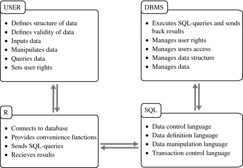
Figure 7.1 How users, R, SQL, DBMS, and databases are related to each other
Let us define some of the terms that we have used up to this point to have a common basis to build upon throughout the remainder of the chapter.
Data are basically a collection of information such as numbers, logical values, text, or some other format. Sometimes collections of information might be data for one purpose but a useless bunch of bits and bytes for another. Imagine that we have collected names of people that have participated in the Olympic Games. If we only care to know who has participated, it might suffice if our data has the format of: ”Carlo Pedersoli”. If, however, we want to sort the data by last name, a format like ”Pedersoli, Carlo” is more appropriate. To be on the safe side, we might even consider splitting the names into first name (”Carlo”) and last name (”Pedersoli”). Being on the safe side plays a crucial role in database design and we will come back to it.
In general a database is simply a collection of data. Within most database systems and relational database systems, the data are related to each other. Consider for example a table that contains the bodyweights of various people. We have at least two types of data in the table: bodyweights and names. What is more, not only does the table store the two variables, but additionally it provides information on how these two pieces of information are related to each other. The most basic rule is this: Every piece of information in a single row is related to each other. We are familiar with handling tables that are structured in this way. In relational databases, these relations between data can be far more complex and will typically be spread across multiple tables.
A database management system (DBMS) is an implementation of a specific database concept bundled together with software. The software is responsible for managing the user rights and access, the way data and meta information are stored physically, or how SQL statements are interpreted and executed. DBMS are numerous and exist as open source as well as commercial products for all kinds of purposes, operation systems, data sizes, and hardware architectures.
Relational database management systems (RDBMS) are a specific type of DBMS based on the relational model and the most common form of database management systems. Relational databases have been around for a while. The concept goes back to the 1970s when Edgar F. Codd proposed to store data in tables that would be related and the relations again stored in tables (Codd 1970). Relational databases, although simple in their conceptual basics, are general and flexible enough to store all kinds of different data structures, while the specific parts of the database remain easy to understand. Popular relational DBMS are Oracle, MySQL, Microsoft SQL Server, PostgreSQL, DB2, Microsoft Access, Sybase, SQLite, Teradata, and File-Maker.1 In this book we exclusively talk about RDBMS and use DBMS and RDBMS interchangeably.
SQL2 is a language to communicate with relational database management systems. When Codd proposed the relational model for databases in 1970, he also proposed to use a language to communicate with database systems that should be general and work only on a meta level. The idea was to be able to express exactly what a DBMS should do—the same statement on different DBMS should always lead to the same result—but leave it completely up to the DBMS how to achieve it computationally (Codd 1970). Such a language would be user friendly and would allow using a common framework for different implementations of the relational model. Based on these conceptual ideas, SQL was later developed by Donald D. Chamberlin and Raymond F. Boyce (1974) and, although occasionally revised throughout the decades, still lives on today as the one common language for relational database communication.
A query is strictly speaking a request sent to a DBMS to retrieve data. In a broader and more frequently used sense it refers to any request made to a DBMS. Such requests might define or manipulate the structure of the data, insert new data, or retrieve data from the database.
7.2 Relational Databases
7.2.1 Storing data in tables
The main concept of relational databases is that any kind of information can be represented in a table. We already know that tables are devices to store data as well as relations—each piece of information within the same row is related to the same entity. To achieve more complex relations—for example, a persons’ weight is measured twice, or the weight is measured for a persons’ children as well—we can relate data from one table to another.
Let us take a look at an example to make this point clear. Imagine that we have collected data on some of our friends—Peter, Paul, and Mary. We collected information on their birthdays, their telephone numbers, and their favorite foods—see Tables 7.1 and 7.2. We had trouble putting the data into one table and ended up separating the data into two tables. Because we do not like to duplicate information, we did not add the full names to the telephone table (Table 7.2), but specified IDs referring to the names in a column called nameid. Now how do we find Peter's telephone number? First, we look up Peter's ID in the birthdays table (Table 7.1) because we know that data on the same line is related—Peter's ID is 1. Second, we check which row in the telephone table has a 1 on nameid—rows one and three. Third, we look up the telephone numbers for these rows—001665443 and 001878345—and realize that Peter has two telephone numbers. We can also reverse the process and ask which name of the birthdays table belongs to a specific telephone number or what number we need to call to speak to a fruit salad or spaghetti lover.
Table 7.1 Our friends’ birthdays and favorite foods
| nameid | name | birthday | favoritefood1 | favoritefood2 | favoritefood3 |
| 1 | Peter Pascal | 01/02/1991 | spaghetti | hamburger | |
| 2 | Paul Panini | 02/03/1992 | fruit salad | ||
| 3 | Mary Meyer | 03/04/1993 | chocolate | fish fingers | hamburger |
The relation in our example is called 1:m or one-to-many, as one person can be related to zero, one, or more telephone numbers. There are of course also 1:1, n:1, and n:m relations (one-to-one, many-to-one, many-to-many), which work just the same way except that the number of data that might show up on one or the other side of the relation differs.
This connection of tables to express relations between data is one of the most important concepts in relational database models. But note that to make it work we had to include identifiers in both tables. These so-called keys ensure that we know which entity the data belongs to and how to combine information from different tables.
Including keys makes some parts of the data redundant—the nameid column exists in Table 7.1 and in Table 7.2—but it also reduces redundancy. Let us consider the example again to make this point clear. Have another look at Table 7.1. There are three columns to store the same type of data. We have to store the data somewhere and what can we do about the fact that some of our friends did name more than one preference? Imagine what it would look like if we recorded more than just these 3 preferences, maybe 5 or 7 or even 10. We would have to add another column for each preference and if somebody only had one preference all the other columns would remain empty. Clearly there has to be another way to cope with this kind of data rather than adding column after column to store some more preferences. Indeed there is.
Table 7.2 Our friends’ telephone numbers
| telephoneid | nameid | telephonenumber |
| 1 | 1 | 001665443 |
| 2 | 2 | 00255555 |
| 3 | 1 | 001878345 |
We divide the data contained in the birthdays table into two separate tables that are related to each other via a key. Have a look at Tables 7.3 and 7.4 for the result. Now we do not have to care how many favorite foods somebody names, because we always have the option of adding another row whenever necessary and still all preferences are unambiguously related to one person.
Table 7.3 Our friends’ birthdays—revised
| name id | first name | last name | birthday |
| 1 | Peter | Pascal | 01/02/1991 |
| 2 | Paul | Panini | 02/03/1992 |
| 3 | Mary | Meyer | 03/04/1993 |
Table 7.4 Our friends’ food preferences
| nameid | foodname | rank |
| 1 | spaghetti | 1 |
| 1 | hamburger | 2 |
| 2 | fruit salad | 1 |
| 3 | chocolate | 1 |
| 3 | fish fingers | 2 |
| 3 | hamburger | 3 |
Even though the data are stored in a cleaner way, we still have some redundancy in our food preference table. Is it necessary to have hamburgers in the table twice? In our example it does not change much, but if the example was just a little more complex, for example, with 10 instead of 3 friends and 80% of them being fans of hamburgers, the table would grow quickly. What if we would like to add further information on the food types? Do we store it in the same table—repeating the information for hamburger over and over again? No, we would do something similar to what we did when putting telephone numbers in a separate table (Table 7.2). In the new food preference table (Table 7.5) all information on the preferences itself remains untouched, because this will be the table on preferences. Furthermore, the key relating it to the birthdays table (Table 7.3)—nameid—and the key relating it to the new table on food (Table 7.6)—foodid—are kept.
Table 7.5 Our friend's food preferences—revised
| rankid | nameid | foodid | rank |
| 1 | 1 | 1 | 1 |
| 2 | 1 | 2 | 2 |
| 3 | 2 | 3 | 1 |
| 4 | 3 | 4 | 1 |
| 5 | 3 | 5 | 2 |
| 6 | 3 | 2 | 3 |
Table 7.6 Food types
| foodid | food name | healthy | kcalp100g |
| 1 | spaghetti | no | 0.158 |
| 2 | hamburger | no | 0.295 |
| 3 | fruit salad | yes | 0.043 |
| 4 | chocolate | no | 0.546 |
| 5 | fish fingers | no | 0.290 |
After restructuring our data, we now have a decent database. Take a look at Figure 7.2 to see how the data are structured. In the schema each table is represented by a square. As we can see, there are four tables. Let us call them birthdays, telephone, foodranking, and foodtypes. The upper part of the square gives the name of the table, the column names are listed in the lower part. The double-headed arrows show which tables are related by pointing to the columns that serve as keys—the columns set in bold and the columns set in italics.
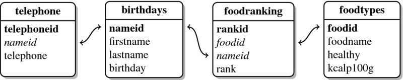
Figure 7.2 Database scheme
The reason why some keys are set in bold and some are set in italics is because there are two types of keys: primary keys and foreign keys. Primary keys are keys that unambiguously identify each row in a table—nameid in our birthdays table (Table 7.3) is an example where each person is associated with exactly one unique nameid. nameid is not a primary key in our telephone table (Table 7.2), as subjects might well have more than one telephone number, making the ID value non-unique. Thus, while nameid in the telephone table is still a key, it is now called a foreign key. Foreign keys are keys that unambiguously identify rows in another table. In other words, each nameid found in the telephone table refers to one and only one row in the birthdays table. There cannot be a nameid in the telephone table that matches more than one nameid in the birthdays table.
Note that it does not matter whether keys consist of one single value per row or a combination of values. Nor does it matter whether the identifier is a number, a string, something else, or a combination of those. A key can span across several columns as long as the value combinations fulfill the requirements for primary or foreign keys. Primary keys in our example are restricted to one single column and are always running integers, but they could look different.
Let us consider an example of an alternative primary key to make this point clear. In our food preference table (Table 7.5) neither nameid nor foodid are sufficient as primary keys, because individuals appear multiple times depending on their stated preferences and the same food might be preferred by several subjects. However, as no one prefers the same food twice, the combination of name identifier and food identifier would be valid as primary key for the food preference table.
7.2.2 Normalization
In the previous paragraphs we decomposed our data step by step. We did so because it saves unnecessary work in the long run and keeps redundancy at bay. Normalization is the process of getting rid of redundancies and possible inconsistencies. In the following section, we will learn about this procedure, which is quite helpful to cope with complex data. If you do not plan to use databases to store data—for example, you only want to store large amounts of data that otherwise fit nicely into a single table, or you only need it for its user management capabilities—you can simply skip this section or come back to it later on.
Let us go through the formal rules for normalization to ensure we understand why databases often look the way they do and how we might do it ourselves. While there are numerous ways of decomposing data stored in tables—called normal forms—we will only cover the first three, as they are the most important and most common.
First normal form
- One column shall refer to one thing and to one thing only and any column row intersection should contain only one piece of data (the atomacy of data requirement).
This rule requires that different types of information are not mixed within one column. One could argue that we violated this rule by storing both first and last names in the name column of our first birthdays table (Table 7.1). We corrected this in the updated birthdays table (Table 7.3), where first name and last name were split up into two columns. Furthermore, it requires that the same data are saved in only one column.
This rule was violated in the first version of our birthdays table, where we had three columns to store a person's favorite food. By exporting the information to the favorite food table (Tables 7.4 and 7.5) and food type table (Table 7.6), this problem was taken care of—a person's favorite food is now stored in a single column. In addition it is not allowed to store more than one piece of the same information in an intersection of row and column. For example, it is not allowed to store two telephone numbers in a single cell of a table. Take a look at Tables 7.7, 7.8, and 7.9 for three examples that violate the first normal form.
- Each table shall have a primary key.
This rule is easy to understand as keys were covered at length in the previous section. It ensures that data can be related across tables and that data in one row is related to the same entity.
Table 7.7 First normal form error—1
| zip code and city |
| 789222 Big Blossom |
| 43211 Little Hamstaedt |
| 123456 Bloomington |
| … |
This table fails the first rule of the first normal form because two different types of information are saved in one column—a city's zip code and a city's name.
Table 7.8 First normal form error—2
| telephone |
| 0897729344, 0666556322 |
| 123123454 |
| 675345334 |
| … |
This table fails the first rule of the first normal form because two telephone numbers are saved within the first row.
Table 7.9 First normal form error—3
| telephone1 | telephone2 |
| 0897729344 | 0666556322 |
| 123123454 | |
| 675345334 | |
| … |
This table fails the first rule of the first normal form because it uses two columns to store the same kind of information.
Second normal Form
- All requirements for the first normal form shall be met.
- Each column of a table shall relate to the complete primary key.
We have learned that a primary key can be a combination of the values of more than one column. This rule requires that all data in a table describe one thing only: only people, only telephone numbers, only food preferences or only food types. One can think of this rule as a topical division of data among tables.
Consider Table 7.10 for a violation of this rule. The primary key of the table is a combination of nameid and foodid. The problem is that firstname and birthday relate to nameid only while favoritefood relates to foodid only. The only column that depends on the whole primary key—the combination of nameid and foodid—is rank, which stores the rank of a specific food in a specific person's food preference order.
A solution to this violation of the second normal form is to split the table into several tables. One table to capture information on persons, one on food and yet another on food preferences. Take a look at Tables 7.3, 7.5, and 7.6 from the previous section for tables that are compliant with the second normal form.
Table 7.10 A second normal form error
| nameid | firstname | birthday | favoritefood | foodid | rank |
| 1 | Peter | 01/02/1991 | spaghetti | 1 | 1 |
| 1 | Peter | 01/02/1991 | hamburger | 2 | 2 |
| 2 | Paul | 02/03/1992 | fruit salad | 3 | 1 |
| 3 | Mary | 03/04/1993 | chocolate | 4 | 1 |
| 3 | Mary | 03/04/1993 | fish fingers | 5 | 2 |
| 3 | Mary | 03/04/1993 | hamburger | 1 | 3 |
This table does not comply to second normal form because all columns except rank either relate to one part of the combined primary key (nameid and foodid) or to other part but not to both.
Third normal form
- All requirements for the second normal form shall be met.
- Each column of a table shall relate only and directly to the primary key.
The third normal form is actually a more strict version of the second normal form. Simply stated, it excludes that data on different things are kept in one table.
Consider Table 7.11. The table only contains three entries, so we could easily use nameid as primary key. Because the primary key only consists of one column, every piece of information depends on the whole primary key. But the table remains odd, because it contains two kinds of information—information related to individuals and information related to food. As the primary key is based on subjects, all information on them relates directly to the primary key. Things look different for information that relates to food. Food-specific information is only related to the primary key insofar as subjects have food preferences. Therefore, including information on food in the table violates the third normal form. Again, the information should be stored in separate tables like in Tables 7.3, 7.5, and 7.6 from the previous subsection.
Table 7.11 A third normal form error
| nameid | firstname | birthday | favoritefood | healthy | kcalp100g |
| 1 | Peter | 01/02/1991 | spaghetti | no | 0.158 |
| 2 | Paul | 02/03/1992 | fruit salad | yes | 0.043 |
| 3 | Mary | 03/04/1993 | chocolate | no | 0.546 |
This table does not comply to third normal form because favoritefood, healthy and kcalp100g do not relate directly to persons which the primary key (nameid) is based on.
Keep in mind that there are several other normal forms, but for our purposes these three should suffice. Recall that normalization is primarily done to ensure data consistency—meaning that any given piece of information is stored only once in a database. If the same piece of information is stored twice, changes would have to be made in multiple places and might contradict each other if forgotten.
There are, however, no technical restrictions that prevent us from putting redundant or inconsistent data structures into a database. Whether this benefits our goal strongly depends on questions like: What purpose does the database serve? What do we describe in our database? How are the elements in our database related to each other? Will information be added in the future? Will the database serve other purposes in the future? How much effort is it to completely normalize our database? The higher the complexity of the data, the higher the number of different purposes a database might serve and the higher the probability that information might be added in the future, the greater the effort that should be put into planning and rigorously designing the database structure. Generally speaking, when you try to extract data from an unknown database, you should always check the structure of the database to make sure you get the right information.
7.2.3 Advanced features of relational databases and DBMS
Understanding how to store data in tables, how to decompose the data, and how relations work in databases is enough for a basic understanding of the nature of databases. But often DBMS have implemented further features like data type definitions, data constraints, virtual tables or views, procedures, triggers, and events that make DBMS powerful tools but go far beyond what can be captured in this short introduction. Nonetheless, we will briefly describe these concepts to provide an idea of what is possible when working with DBMS.
One aspect we usually have to take care of when building up a database is to specify each column's data type. The data type definition tells the DBMS how to handle and store the data; it affects the required disk space and also impacts efficiency. There are several broad data types that are implemented in one way or another in every DBMS: boolean data, that is, true and false values, numeric data (integer and float), character or text data, data referring to dates, times, and time spans as well as data types for files (so-called BLOBs—binary large objects). Which types are available and how they are implemented depends on the specific DBMS, so we will not go into details here. The manual section of each DBMS should list and describe the supported data types, how they are implemented, and further features that are associated with it. To get an idea, consider Table 7.11 once more. Column by column the data types can be specified as: integer, character, date, character, boolean, and float.
Beyond fixing columns to specific types of data, some DBMS even implement the possibility to constrain data. Constraining data enables the user to define under which circumstances—for which values and value ranges—data should be accepted and in which cases the DBMS should reject to store the data. In general, there are two ways to constrain data validity: Specifying columns as primary or foreign keys and explicitly specifying which values or value ranges are valid and which are not. Setting a column as primary key results in the rejection of duplicated values because primary keys must identify each row unambiguously. Defining a column as foreign key will lead to the rejection of values that are not already part of the primary key it relates to. Explicit constraining of data instead is user-defined and might be as simple as forbidding negative values or more complex involving several clauses and references to other tables. No matter which type of constraint is used the general behavior of the DBMS is to reject values that do not fulfill the constraint.
DBMS are designed for consistent handling of data. This entails that queries to the database should not break it, for example, if an invalid change is requested or a data import suddenly breaks up—for example, when our system crashes. This is ensured by enforcing that a manipulation is completely carried out or not at all. Furthermore, DBMS usually provide a way to define transactional blocks. This feature is useful whenever we have a manipulation that takes several steps and we want all steps to take effect or none—that is, we do not want the process to stop halfway through because one statement causes an error, leaving us with data that is partially manipulated.
Nearly all DBMS provide a way to secure access to the database. The simplest possibility is to ask for a password before granting access to the whole database but more elaborate frameworks are common like having several users with their own passwords. Furthermore, each user account can be accompanied with different user rights. One user might only be allowed to read a single table, while another can read all tables and even add new data. Yet other users might be allowed to create new tables and grant user rights to other users.
DBMS can easily handle accesses of more than one user to the same database at the same time. That is, DBMS will always give you the present state of the database as response to a query including changes made by other users but only those that were completely executed. How a DBMS precisely solves problems of concurrent access is DBMS specific.
As the normalization of data and complex structures makes it more cumbersome to assemble the data needed for a specific purpose, most DBMS have the possibility to define virtual tables called views. Imagine that we want to retrieve and compose data from different data tables frequently. We can define a query each time we need the specific combination of data. Alternatively, we can define the query once and save it in a separate table. The downside of this operation is that it takes up additional disk space. Further, we have to recreate the table each time to make sure it is up to date, which is identical to defining the query anew each time we need the specific combination of data.
Another, more elegant solution is to store the query that provides the data we need as a virtual table. This table is virtual because instead of the data only the query that provides the data is stored. This virtual table behaves exactly as if the data was stored in the table, but potentially saves a lot of rewriting and rethinking. Compared to executing the query once and saving the results in the database, the data in the virtual table will always be up to date.
All DBMS provide functions for data manipulation and aggregation in addition to the simple data storage capacities. These functions might provide us with the current date, the absolute value of a number, a substring, the mean for a set of values, and so on. Note that while R functions can return all kinds of data formats, database functions are restricted to scalars. Which functions are provided and how they are named is DBMS dependent. Furthermore, most DBMS allow user-defined functions as well but, again, the syntax for function definition might vary.
Another DBMS-dependent feature is procedures and triggers. Procedures and triggers help extending the functionality of SQL. Imagine a database with a lot of tables, where adding a new entry involves changes to many tables. Procedures are stored sequences of queries that can be recalled whenever needed, thus making repeating tasks much easier. While procedures are executed upon user request, triggers are procedures that are executed automatically when certain events, like changes in a table, take place.
7.3 SQL: a language to communicate with Databases
7.3.1 General remarks on SQL, syntax, and our running example
Now that we have learned how databases and DBMS work and which features they provide, we can turn our attention to SQL, the language to communicate with DBMS. SQL is a multipurpose language that incorporates vocabulary and syntax for various tasks:
- DCL (data control language)
The DCL part of SQL helps us to define who is allowed to do what and where in our database and allows for fine-grained user rights definitions.
- DDL (data definition language)
DDL is the part of SQL that defines the structure of the data and its relations. This means that the vocabulary enables us to create tables and columns, define data types, primary keys and foreign keys, or to set constraints.
- DML (data manipulation language)
The DML part of SQL takes care of actually filling our database with data or retrieving information from it.
- TCL (transaction control language)
The last part of SQL is TCL, which enables us to commit or rollback previous queries. This is similar to save and undo buttons in ordinary desktop programs.
The syntax and vocabulary of SQL is rather simple. Let us first consider the general syntax before moving on to specific vocabularies and syntaxes of the different language branches of SQL.
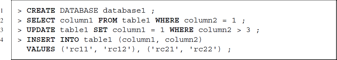
SQL statements generally start with a command describing which action should be executed—for example, CREATE, SELECT, UPDATE, or INSERT INTO—followed by the unit on which it should be executed—for example, FROM table1—and one or more clauses—for example, WHERE column1 = 1. Below you find four SQL statement examples.
Although it is customary to write all SQL statements in capital letters, SQL is actually case insensitive towards its key words. Using capital or small case does not change the interpretation of the statements. Note however, that depending on the DBMS, the DBMS might be case sensitive to table and column names. For purposes of readability we will stick to the capitalized key words and lower case table and column names.
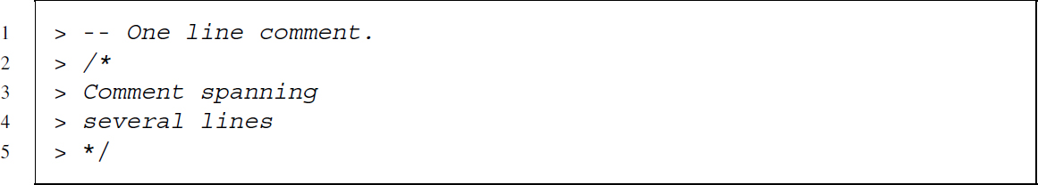
Each SQL statement ends with a semicolon—therefore, SQL statements might span across multiple lines.
Comments either start with -- or have to be put in between /* and */.
For the remainder of this section we will use the birthdays, foodranking, and foodtypes tables (Tables 7.3, 7.5, and 7.6) from the database that we built up in the previous sections. As SQL is the common standard for a broad range of DBMS, the examples should work with most DBMS that speak SQL. However, there might always be slight differences—for example, SQLite does not support user management.
To access the database, you can either use R as client—you will find a description of the possible ways in the next section—or install and use another client software. Before you can access the database, you have to create your own server—except when using SQLite, which works with the R package RSQLite out of the box. We recommend using a MySQL community server in combination with MySQL Workbench CE for a start. Both the MySQL server and MySQL Workbench are easy to install, easy to use, and can be downloaded free of charge. Furthermore, MySQL ODBC drivers are reliable, are available for a large range of platforms, and it is easy to connect to the server from within R by making use of RODBC.3
7.3.2 Data control language—DCL
To control access and privileges to our database, we first ask the DBMS to create a database called db1:

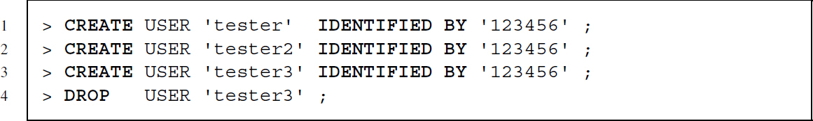
Next, we create and delete several users identifying themselves by password:
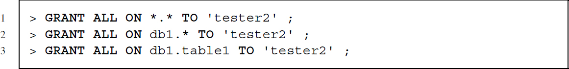
Now we can use two powerful SQL commands to define what a user is allowed to do. GRANT for granting privileges and REVOKE to remove privileges. A full SQL statement granting user tester all privileges; all privileges for a certain database, and all privileges for a certain table in a database looks as follows:
We can also grant specific privileges only, for example, for selecting and inserting information:

We can add the right to grant privileges to other users as well:

To remove all privileges from our test user, we can use REVOKE or delete the user altogether.

7.3.3 Data definition language—DDL
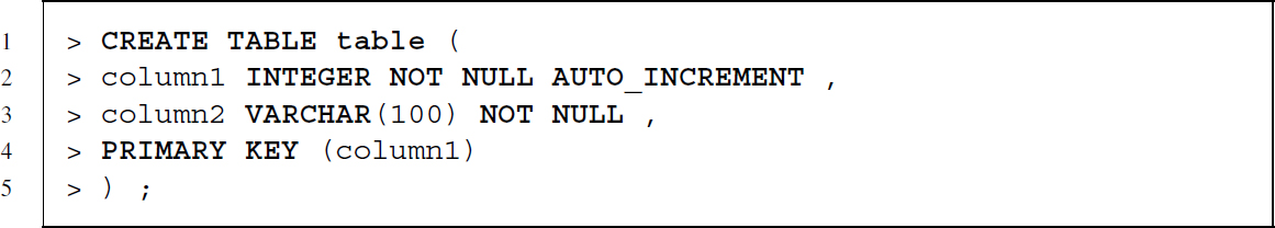
After having created a database and a user and having set up the user rights, we can turn to those statements that define the structure of our data. The commands for data definition are CREATE TABLE for the definition of tables, ALTER TABLE for changing aspects of an existing table, and DROP TABLE to delete a table from the database. Let us start by defining Table 7.3, the revised birthdays table.
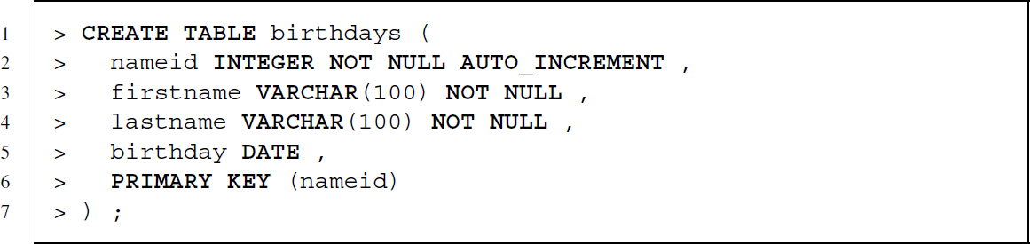
Let us go through this line by line. The first line starts the statement by using CREATE TABLE to indicate that we want to define a new table and also specifies the name ‘birthdays’ for this new table. The details of the columns follow in parentheses. Each column definition is separated by a colon and always starts with the name of the column. After the name we specify the data type and may add further options. While the data types of nameid and birthday—INTEGER and DATETIME—are self-explaining, the name variables were defined as characters with a maximum length of 100 characters—VARCHAR(100).
Using the options NOT NULL and AUTO_INCREMENT we define some basic constraints. NOT NULL specifies that this column cannot be left empty—we demand that each person included in birthdays has to have a name identifier, a first name and a last name. Should we try to add an observation to the table without all of these pieces of information, the DBMS will refuse to include it in birthdays. The AUTO_INCREMENT parameter for the nameid column adds the option that whenever no name identifier is manually specified when inserting data, the DBMS takes care of that by assigning a unique number. The last line before we close the parentheses and terminate the statement with a semicolon adds a further constraint to the table. With PRIMARY KEY (nameid) we define that nameid should serve as primary key. The DBMS will prevent the insertion of duplicated values into this column.
Let us add two more tables to our database to add some complexity and to showcase some further concepts. We define the structure of Tables 7.5 and 7.6, where we recorded food preferences and food attributes.
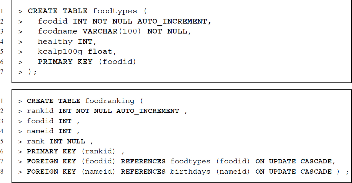
The creation of foodtypes is quite similar to that of birthdays. More interesting is the creation of the food preference table, because it relates to data about subjects as well as to information about food—captured in birthdays and foodtypes. Take a look at the lines starting with FOREIGN KEY. First, we choose the column that serves as foreign key, then we define which primary key this column refers to, followed by further options. By specifying ON UPDATE CASCADE we choose that whenever the primary key changes, this change is cascaded down to our foreign key column that is changed accordingly.
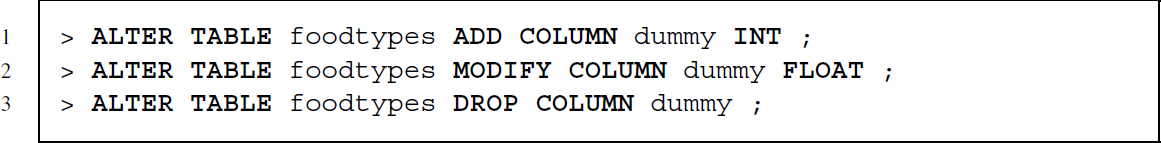
To change the definition of a table later on, we can make use of the ALTER TABLE command. Below you find several examples for adding a column, changing the data type of this column, and dropping it again.
To get rid of a table, we can use DROP TABLE.

7.3.4 Data manipulation language—DML
Now that we have defined some tables in our database, we need to learn how to insert, manipulate, and retrieve data from it. Figure 7.3 provides an overview of the structure of our database—bold column names refer to primary keys while italics denote foreign keys; the arrows show which foreign keys relate to which primary keys.
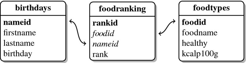
Figure 7.3 SQL example database scheme
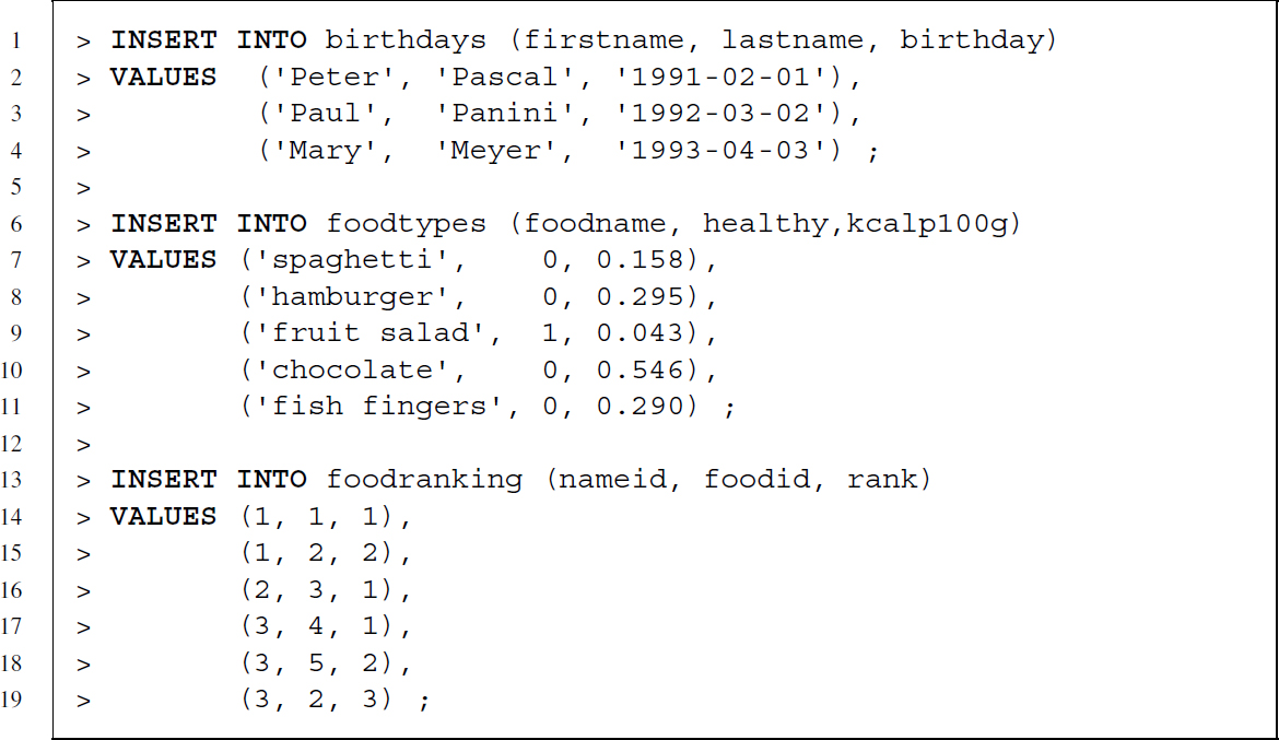
The following three SQL statements use the INSERT INTO command to fill our tables with data. After selecting the name of the table to fill, we also specify column names—enclosed in parentheses—to specify for which columns data are provided and in which order. If we had not specifed column names, data for all columns would be provided in the same order as in the definition of the table. As each table contains one column that is automatically filled with identification numbers—nameid, foodid, rankid—we do not want to specify this information manually but let the DBMS take care of it. Note that every non-numeric value—text and dates—is enclosed in single quotes'.
To update and delete rows of data, we have to specify for which rows the update or deletion takes place. For this we can make use of the WHERE clause. Let us create a new column that captures whether or not the energy of a food type is above 0.2 kcal per 100 g. To achieve this, we tell the DBMS to create a new column and to update the column.4 In a last step, we delete the column again:
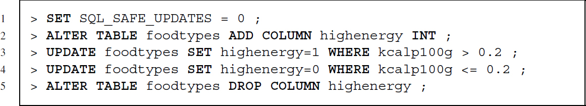
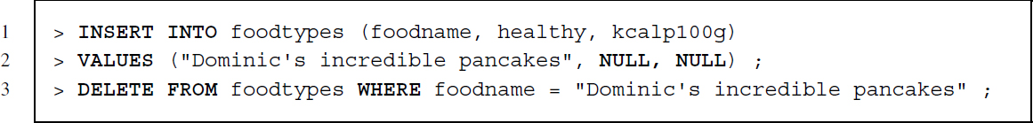
Let us have another example of deleting data. We first create a row with false data and then drop the row:
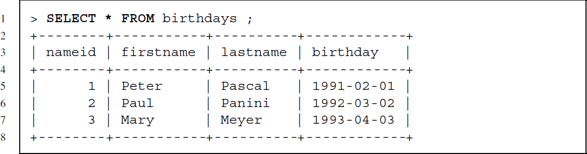
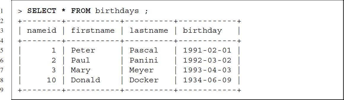
Data retrieval works similar to insertion of data and is achieved using the SELECT command. After the SELECT command we specify the columns we want to retrieve, followed by the keyword FROM and the name of the table from which we want to get the data. The following query retrieves all columns of the birthday table:
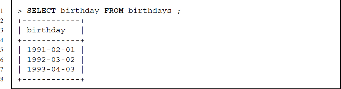
This retrieves only the birthdays:
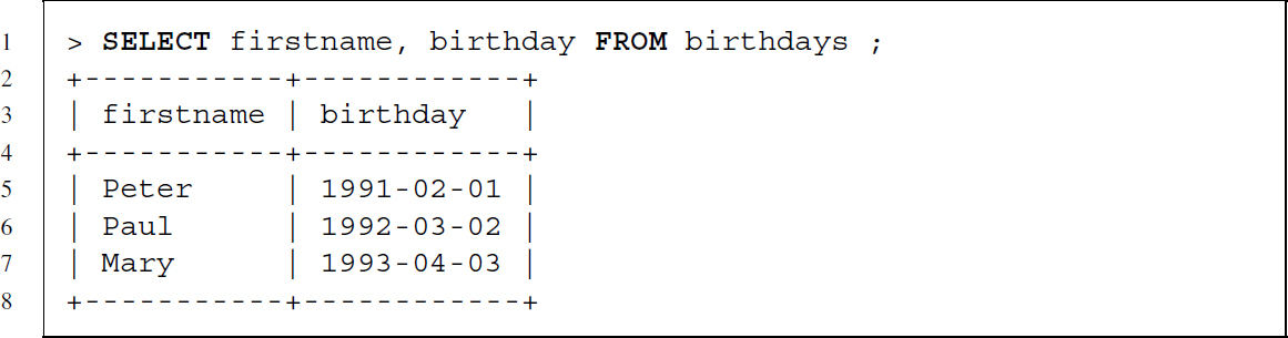
Retrieving birthdays and first names:
So far we only retrieved data from a single table but often we need to combine data from multiple tables. Combining data is done with the JOIN command—similar to the merge() function in R. There are four possible joins:5
- INNER JOIN will return a row whenever there is a match in both tables.
- LEFT JOIN will return a row whenever there is a match in the first table.
- RIGHT JOIN will return a row whenever there is a match in the second table.
- FULL JOIN will return a row whenever there is a match in one of the tables.
To show how joins work, let us consider three examples in which data from the birthdays table and the foodranking table are combined. Both tables are related by nameid. We will match rows on this identifier, meaning that information from both tables is merged by identical values on nameid.
To show the differences in the join statements, let us add a row to the birthdays table with a nameid value that is not included in the foodranking table:

The birthdays table now has one additional row:
Recall the food ranking table (Table 7.5). The first JOIN command is an inner join, which needs matching keys in both tables. Therefore, only information related to Peter, Paul, and Mary should show up in the resulting table, because Donald does not have a nameid in both tables:
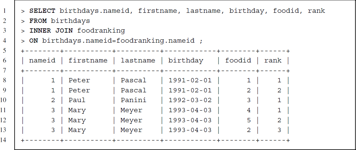
Joins are de facto extended SELECT statements. As in an ordinary SELECT statement we first specify the command followed by the names of the columns to be retrieved. Note that the columns to be retrieved can be from both tables. If columns with the same name exist in both tables they should be preceded by the table name to clarify which column we are referring to—for example, birthdays.nameid refers to the name identification column in the birthdays table. The column specification is followed by FROM and the name of the first table. In contrast to ordinary SELECT statements we now specify the join keywords—in this case INNER JOIN—followed by the name of the second table. Using the keyword ON we specify which columns serve as keys for the match.
As expected, Donald does not show up in the resulting table because his id is not included in the foodranking table. Furthermore, the resulting table has a row for each food preference so that information from the birthdays table like name and birthday is duplicated as needed.
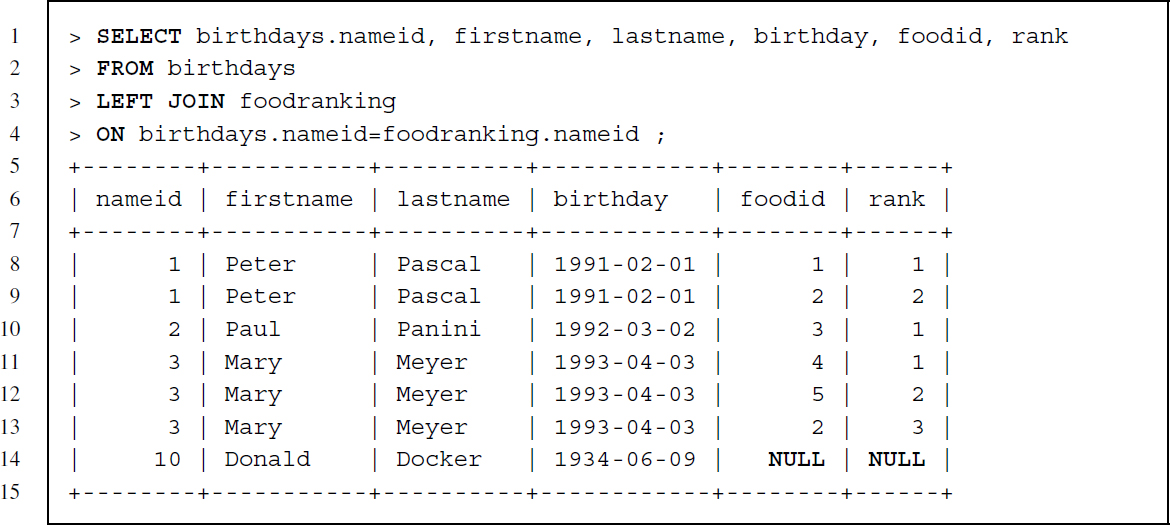
Because LEFT JOIN only requires that a key appears in the first—or left—table, Donald Docker is now included in the resulting table, but there is no information on food preference—both columns show NULL values for Donald Docker. If we had specified the join the other way around with foodranking being the first table and birthdays second, Donald would not have been included as his id is not part of foodranking.
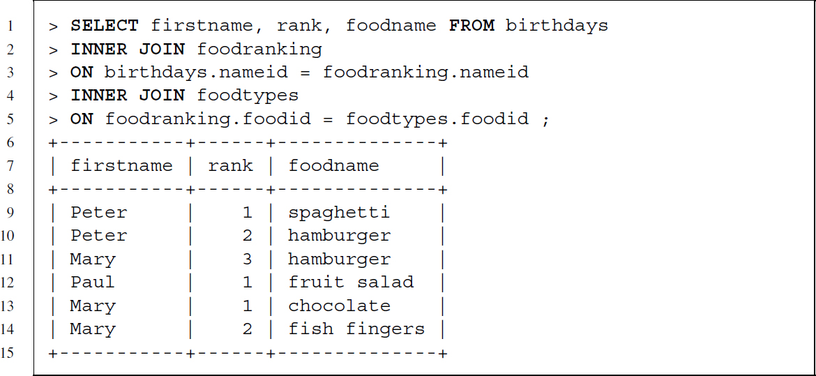
More than one table can be combined with join statements. To get the individuals’ preferences as well as the actual name of the food—we need columns from three tables. We gather this information by extending the INNER JOIN of our previous example with another join that specifies that tables foodranking and foodtypes are related via their foodid columns and a request for the foodname column:
Let us clean up before moving to the next section by dropping the data on Donald from the database:

7.3.5 Clauses
We have already used the WHERE clause in SQL statements to restrict data manipulations to certain rows, but we have neither treated the clause thoroughly nor have we mentioned that SQL also has other clauses.
Let us begin by extending our knowledge of the WHERE clause. We already know that it restricts data manipulations and retrievals to specific rows. Restrictions are specified in the form of column_name operator value, where operator defines the type of comparison and value, the content of the comparison. Possible operators are = and != for equality/inequality, <, <=, >, >= for smaller (or equal) and greater (or equal) values, LIKE for basic matching of text patterns and IN to specify a set of acceptable values.
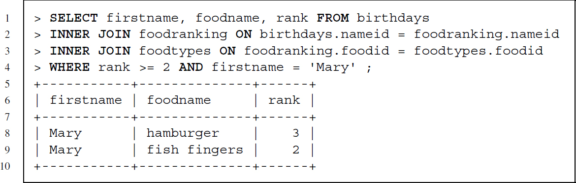
We can also use AND and OR to build more complex restrictions and even nest restrictions by using parentheses. Let us start with a composite WHERE clause with two conditions—see the code snippet below. This statement retrieves data from all three tables but the resulting set of rows is restricted by the WHERE clause to those lines that have a food preference rank equal or larger than 2 and where the firstname matches ’Mary’.
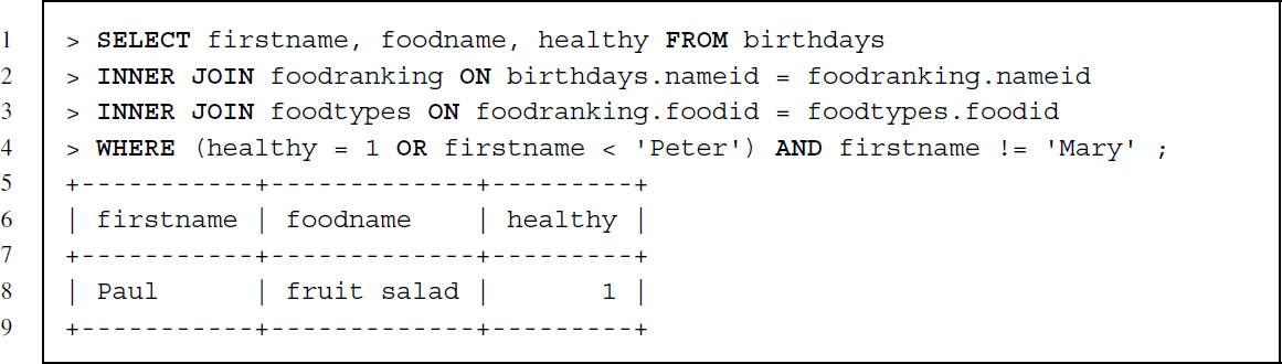
The next statement has a nested composite WHERE clause and uses alphabetical sorting of text (firstname < ’Peter’). While firstname should never match ’Mary’, the other part of the clause states that either healthy should equal to 1 or firstname should be a string that precedes Peter alphabetically.
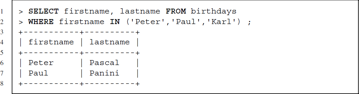
The following statement is an example of using IN—the value of firstname should match one of three names:
The last statement showcases the usage of LIKE—% is a wildcard for any number of any character and _ is a wildcard for any one character. The statement requires that a row is part of the resulting table if either firstname contains er at the end of the string preceded by any number of characters or that lastname contains an e that is preceded by any number of characters and followed by exactly one character.

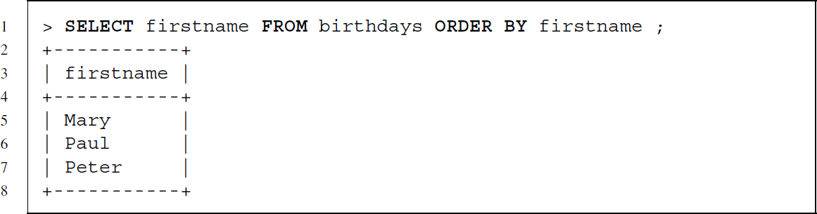
A second clause is the ORDER BY clause, which enables us to order results by column values. Below you find several examples that order the results of a data retrieval. The standard for sorting is to do it in ascending order.
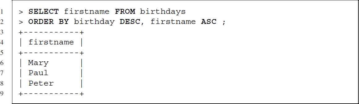
To revert this behavior, we can add the keyword DESC. We can also specify more than one column to define the sort order and choose for every column whether it should be used in ascending or descending order.
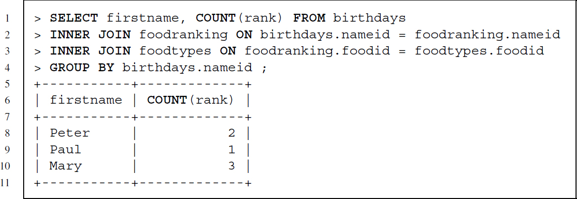
The GROUP BY clause allows aggregating values. The type of aggregation depends on the specific aggregation function that we use.6 In the following example the use of GROUP BY is exemplified with the COUNT aggregation function, which returns a count of how many food preferences each person has—the result is a table with a row for each unique nameid from the birthdays table and a count of how many times a food preference was recorded.
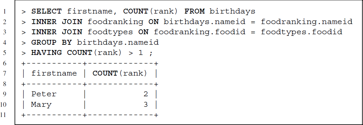
To filter the aggregation table resulting from a GROUP BY clause, a special clause is needed—a WHERE clause can be used in combination with GROUP BY, but this excludes rows only before aggregation not after. Using HAVING we can filter the aggregation results.
7.3.6 Transaction control language—TCL
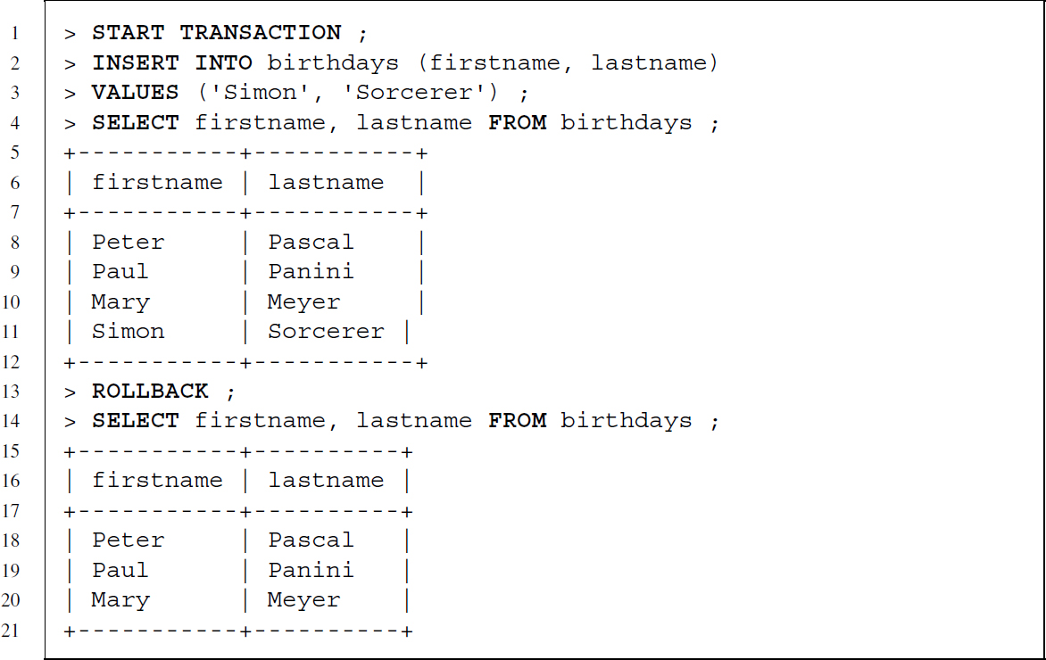
SQL statements are usually executed after a statement is sent to the DBMS and made permanent unless some error occurs. This standard behavior can be modified by explicitly starting a transacting with START TRANSACTION. Using this statement a save point is created. Instead of executing each SQL statement immediately and making them permanent, each statement is executed temporarily until it is explicitly committed by the user with the COMMIT command. If an error occurs before COMMIT was specified all changes until the last save point are reversed.
We can achieve the same behavior by asking the DBMS to ROLLBACK until the last save point. Below you find an example where some data are added and then the database is reversed to the status when the save point was set.
7.4 Databases in action
7.4.1 R packages to manage databases
R has several packages to connect to DBMS: One way is to use packages that rely on the DBI package (R Special Interest Group on Databases 2013) like RMySQL (James and DebRoy 2013), ROracle (Denis Mukhin and Luciani 2013), RPostgreSQL (Conway et al. 2013) and RSQLite (James and DebRoy 2013) to establish a “native” connection to a specific DBMS. While the DBI package defines virtual functions, the database-specific packages implement these functions in database-specific ways. The added value of this approach is that while there is a common set of functions that are expected to work the same way, different package authors can concentrate on developing and maintaining solutions for one type of database only.
Another approach to work with DBMS via R is to rely on RODBC (Ripley and Lapsley 2013). This package uses open database connectivity (ODBC) drivers as an indirect way to connect to DBMS and requires that the user installs and configures the necessary driver before using it in R. ODBC drivers are available across platforms and for a wide variety of DBMS. They even exist for data storage formats that are no databases at all, like CSV or XLS/XLSX. The package also delivers a general approach to manage different types of databases with the same set of functions. On the downside, this approach depends on whether ODBC drivers are available for the DBMS type to be used in combination with the platform R is working on.
Which package to use is essentially a matter of taste and how difficult it is to get the package or driver running—at the moment and to the authors’ best knowledge RSQLite is the only package that works completely out of the box across multiple platforms. All other packages need driver installation and/or package compilation.
7.4.2 Speaking R-SQL via DBI-based packages
As the DBI package defines a common framework for working with databases from within R, all database packages that rely on this framework work the same way, regardless of which particular DBMS we establish a connection to. To show how things work for DBI-based packages, we will make use of RSQLite. Let us load the birthdays database, which has been bundled as an SQLite file and execute a simple SELECT statement:
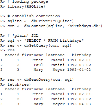
Using these functions we are able to perform basic database operations from within R. Let us go through the code line by line. First we load the RSQLite package so that R knows how to handle SQLite databases. Next, we build up a connection to the database by first defining the driver and then using the driver in the actual connection. Because our SQLite database has no password, we do not have to specify much except the database driver and the location of the database. Now we can query our database. We have two functions to do so: dbGetQuery() and dbSendQuery(). Both functions ask the DBMS to execute a single query, but differ in how they handle the results returned by the DBMS. The first one fetches all results and converts them to a data frame, while the second one will not fetch any results unless we explicitly ask R to do so with the fetch() function.
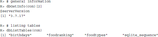
Because we can send any SQL query that is supported by the specific DBMS, these four functions suffice to fully control databases from within R. Nonetheless, there are several other functions provided by DBI-based packages. These functions do not add further features but help to make communication between R and DBMS more convenient. There are, for example, functions for getting an overview of the database properties—dbGetInfo()—and the tables that are provided—dbListTables():
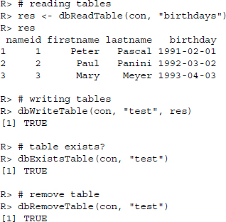
There are also functions for reading, writing, and removing tables, which are as convenient as they are self-explanatory: dbReadTable(), dbWriteTable(), dbExistsTable(), and dbRemoveTable().
To check the data type an R object would be assigned if stored in a database, we use dbDataType():
R> # checking data type
R> dbDataType(con, res$nameid)
[1] ”INTEGER”
R> dbDataType(con, res$firstname)
[1] ”TEXT”
R> dbDataType(con, res$birthday)
[1] ”TEXT”
We can also start, revert, and commit transactions as well as close a connection to a DBMS:
R> # transaction management
R> dbBeginTransaction(con)
[1] TRUE
R> dbRollback(con)
[1] TRUE
R> dbBeginTransaction(con)
[1] TRUE
R> dbCommit(con)
[1] TRUE
R> # closing connection
R> dbDisconnect(con)
[1] TRUE
7.4.3 Speaking R-SQL via RODBC
Communicating with databases by relying on the RODBC package is quite similar to the DBI-based packages. There are functions that forward SQL statements to the DBMS and convenience functions that do not require the user to specify SQL statements.7
Let us start by establishing a connection to our database and passing a simple SELECT * statement to read all lines of the birthdays table:
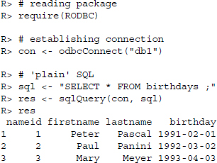
The code to establish a connection and pass the SQL statement to the DBMS is quite similar to what we have seen before. One difference is that we do not have to specify any driver as the driver and all other connection information have already been specified in the ODBC manager so that we only have to refer to the name we gave this particular connection in the ODBC manager.
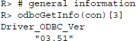
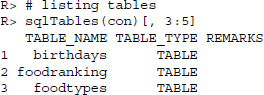
Besides the direct execution of SQL statements, there are numerous convenience functions similar to those found in the DBI-based packages. To get general information on the connection and the drivers used or to list all tables in the database, we can use odbcGetInfo() and sqlTables():
To get an overview of the ODBC driver connections that are currently specified in our ODBC manager, we can use odbcDataSources(). The function reveals that db1 to which we are connected is based on MySQL drivers version 5.2:
![]()
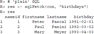
We can also ask for whole tables without specifying the SQL statement by a simple call to sqlFetch():
Similarly, we can write R data frames to SQL tables with convenience functions. We can also empty tables or delete them altogether:
R> # writing tables
R> test <- data.frame(x = 1:3, y = letters[7:9])
R> sqlSave(con, test, ”test”)
R> sqlFetch(con, ”test”)
x y
1 1 g
2 2 h
3 3 i

R> # empty table
R> sqlClear(con, ”test”)
R> sqlFetch(con, ”test”)
[1] x y
<0 rows> (or 0-length row.names)

R> # drop table
R> sqlDrop(con, ”test”)
Summary
In this chapter we learned about databases, SQL, and several R packages that enable us to connect to databases and to access the data stored in them. Simply put, relational databases are collections of tables that are related to one another by keys. Although R is capable of handling data, databases offer solutions to certain data management problems that are best dealt with in a specific environment. SQL is the lingua franca for communication between the user and a wide range of database management systems. While SQL allows us to define what should be done, it is in fact the DBMS that manages how this is achieved in a reliable manner. As a multipurpose language we can use SQL to manage user rights, define data structures, import, manipulate, and retrieve data as well as to control transactions. We have seen that R is capable of communicating with a variety of databases and provides additional convenience functions. As DBMS were designed for reliable and efficient handling of data they might be solutions to limited RAM size, multipurpose usages of data, multiuser access to data, complex data storage, and remote access to data.
Further reading
Relational databases and SQL are part of the web technology community and are therefore treated in hundreds of forums, blogs, and manuals. Therefore, you can easily find a solution to most problems by typing your question into any ordinary search engine. To learn the full spectrum of options for a specific DBMS, you might be better advised to turn to a comprehensive treatment of the subject. For an introduction to MySQL we recommend Beaulieu (2009). Those who like it a little bit more fundamental might find the SQL Bible (Kriegel and Trukhnov 2008) or Relational Database Design and Implementation (Harrington 2009) helpful sources. Last but not least the SQL Pocket Guide (Gennick 2011) is a gentle pocket reference that fits in every bookshelf.
Problems
The following problems are built around two—more or less—real-life databases, one on Pokemon characters, the other on data about elections, governments, and parties. The Pokemon data was gathered and provided by Francisco S. Velazquez. We extracted some of the tables and provide them as CSV files along with supplementary material for this chapter. The complete database is available at https://github.com/kikin81/pokemon-sqlite. The ParlGov database is provided by Döring (2013). It combines data on “elections, parties, and governments for all EU and most OECD members from 1945 until today” gathered from multiple sources. More information is available at http://parlgov.org. Downloading the whole database will be part of the exercise.
Pokemon problems
-
Load the RSQLite package and create a new RSQLite database called pokemon.sqlite.
-
Use read.csv2() to read pokemon.csv, pokemon_species.csv, pokemon_stats.csv, pokemon_types.csv, stats.csv, type_efficacy.csv, and types.csv into R and write the tables to pokemon.sqlite. Have a look at PokemonReadme.txt to learn about the tables you imported.
-
Use functions from DBI/RSQLite to read the tables that you stored in the database back into R and save them in objects named: pokemon, pokemon_species, pokemon_stats, pokemon_types, stats, type_efficacy, and types.
-
Build a query that SELECTs those pokemon from table pokemon that are heavier than 4000. Next, build a SELECT query that JOINs tables pokemon and pokemon_species.
-
Combining the previous SQL queries, build a query that JOINs both tables and restricts the results to Pokemon that are heavier than 4000.
-
Build a query that SELECTs all Pokemon names from table pokemon_species that have Nido as part of their name.
-
Fetching names.
- Build a query that SELECTs Pokemon names.
- Send the query to the database using dbSendQuery() and save the result in an object.
- Use fetch() three times in a row, each time retrieving another set of five names.
- Use dbClearResult() to clean up afterwards.
-
Creating views.
- Create a VIEW called pokeview …
- … that JOINs table pokemon with table pokemon_species,
- … and contains the following information: height and weight, species identifier, Pokemon id from which the Pokemon evolves, the id of the evolution chain, and ids for Pokemon and species.
- Create a VIEW called typeview …
- … that JOINs pokemon_types and types …
- … and contains the following information: slot of the type, identifier of the type, and ids for Pokemon, damage class, and type.
- Create a VIEW called statsview …
- … that JOINs pokemon_stats and stats …
- … and contains the following information: identifier of the statistic, base value of the statistics, and ids for Pokemon, statistics, and damage class.
-
Using the views you created, which Pokemon are of type dragon? Which Pokemon has most health points, which has the best attack, defense, and speed?
ParlGov problems
-
Use download.file() with mode=”wb” to save the following resource http://parlgov .org/stable/static/data/parlgov-stable.db as parlgov.sqlite and establish a connection.
-
Get a list of all tables in the database. According to info_data_source, which external data sources were used for the database?
-
Figure out for which countries the database offers data.
-
Which time span is covered by the election table?
-
How many early elections were there in Spain, the United Kingdom, and Switzerland?
-
Creating views.
- CREATE a VIEW named edata …
- … that JOINs table election_result …
- … with tables election, country, and party …
- … so that the view contains the following information: country name, date of the election, the abbreviated party name, party name in English, seats to be won in total, seats won by party, vote share won by the party, as well as ids for country, election, election results, and party.
- Make sure the VIEW is restricted to elections of type 13 (elections to parliament).
- Read the data of the view into R and save it in an object.
- Add a variable storing the seat share.
- Plot vote shares versus seat shares. Use text() to add the name of the country if vote share and seat share differ by more than 20 percentage points.
-
Find answers to the following questions in the database.
- Which country had a cabinet lead by Lojze Peterle?
- Which parties were part of that government?
- What were their vote shares in the election?
-
More SELECT queries.
- Build a query that SELECTs column tbl_name and type from table sqlite_master.
- Build a query that SELECTs column sql from table sqlite_master WHERE column tbl_name equals edata. Save the result in an object and use cat() to display the contents of the object.
- Do the same for tbl_name equal to view_election.